Deep Markov Model
Introduction
We’re going to build a deep probabilistic model for sequential data: the deep markov model. The particular dataset we want to model is composed of snippets of polyphonic music. Each time slice in a sequence spans a quarter note and is represented by an 88-dimensional binary vector that encodes the notes at that time step.
Since music is (obviously) temporally coherent, we need a model that can represent complex time dependencies in the observed data. It would not, for example, be appropriate to consider a model in which the notes at a particular time step are independent of the notes at previous time steps. One way to do this is to build a latent variable model in which the variability and temporal structure of the observations is controlled by the dynamics of the latent variables.
One particular realization of this idea is a markov model, in which we have a chain of latent variables, with each latent variable in the chain conditioned on the previous latent variable. This is a powerful approach, but if we want to represent complex data with complex (and in this case unknown) dynamics, we would like our model to be sufficiently flexible to accommodate dynamics that are potentially highly non-linear. Thus a deep markov model: we allow for the transition probabilities governing the dynamics of the latent variables as well as the the emission probabilities that govern how the observations are generated by the latent dynamics to be parameterized by (non-linear) neural networks.
The specific model we’re going to implement is based on the following reference:
[1] Structured Inference Networks for Nonlinear State Space Models, Rahul G. Krishnan, Uri Shalit, David Sontag
Please note that while we do not assume that the reader of this tutorial has read the reference, it’s definitely a good place to look for a more comprehensive discussion of the deep markov model in the context of other time series models.
We’ve described the model, but how do we go about training it? The inference strategy we’re going to use is variational inference, which requires specifying a parameterized family of distributions that can be used to approximate the posterior distribution over the latent random variables. Given the non-linearities and complex time-dependencies inherent in our model and data, we expect the exact posterior to be highly non-trivial. So we’re going to need a flexible family of variational distributions if we hope to learn a good model. Happily, together PyTorch and Pyro provide all the necessary ingredients. As we will see, assembling them will be straightforward. Let’s get to work.
The Model
A convenient way to describe the high-level structure of the model is with a graphical model.
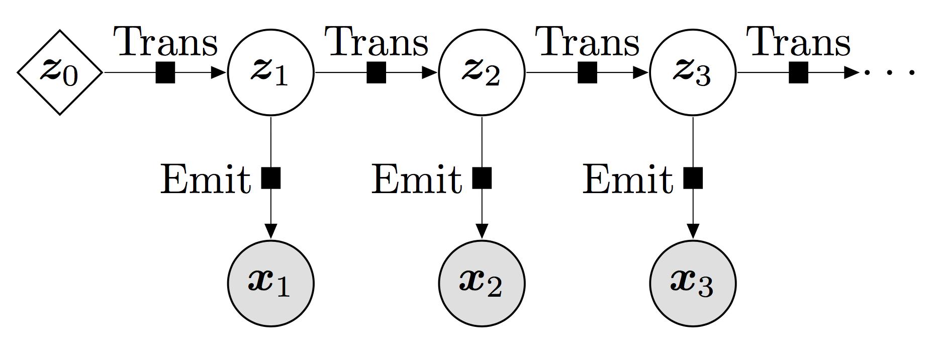
Here, we’ve rolled out the model assuming that the sequence of observations is of length three: \(\{{\bf x}_1, {\bf x}_2, {\bf x}_3\}\). Mirroring the sequence of observations we also have a sequence of latent random variables: \(\{{\bf z}_1, {\bf z}_2, {\bf z}_3\}\). The figure encodes the structure of the model. The corresponding joint distribution is
Conditioned on \({\bf z}_t\), each observation \({\bf x}_t\) is independent of the other observations. This can be read off from the fact that each \({\bf x}_t\) only depends on the corresponding latent \({\bf z}_t\), as indicated by the downward pointing arrows. We can also read off the markov property of the model: each latent \({\bf z}_t\), when conditioned on the previous latent \({\bf z}_{t-1}\), is independent of all previous latents \(\{ {\bf z}_{t-2}, {\bf z}_{t-3}, ...\}\). This effectively says that everything one needs to know about the state of the system at time \(t\) is encapsulated by the latent \({\bf z}_{t}\).
We will assume that the observation likelihoods, i.e. the probability distributions \(p({{\bf x}_t}|{{\bf z}_t})\) that control the observations, are given by the bernoulli distribution. This is an appropriate choice since our observations are all 0 or 1. For the probability distributions \(p({\bf z}_t|{\bf z}_{t-1})\) that control the latent dynamics, we choose (conditional) gaussian distributions with diagonal covariances. This is reasonable since we assume that the latent space is continuous.
The solid black squares represent non-linear functions parameterized by neural networks. This is what makes this a deep markov model. Note that the black squares appear in two different places: in between pairs of latents and in between latents and observations. The non-linear function that connects the latent variables (‘Trans’ in Fig. 1) controls the dynamics of the latent variables. Since we allow the conditional probability distribution of \({\bf z}_{t}\) to depend on \({\bf z}_{t-1}\) in a complex way, we will be able to capture complex dynamics in our model. Similarly, the non-linear function that connects the latent variables to the observations (‘Emit’ in Fig. 1) controls how the observations depend on the latent dynamics.
Some additional notes: - we can freely choose the dimension of the latent space to suit the problem at hand: small latent spaces for simple problems and larger latent spaces for problems with complex dynamics - note the parameter \({\bf z}_0\) in Fig. 1. as will become more apparent from the code, this is just a convenient way for us to parameterize the probability distribution \(p({\bf z}_1)\) for the first time step, where there are no previous latents to condition on.
The Gated Transition and the Emitter
Without further ado, let’s start writing some code. We first define the two PyTorch Modules that correspond to the black squares in Fig. 1. First the emission function:
class Emitter(nn.Module):
    """
    Parameterizes the bernoulli observation likelihood p(x_t | z_t)
    """
    def __init__(self, input_dim, z_dim, emission_dim):
        super().__init__()
        # initialize the three linear transformations used in the neural network
        self.lin_z_to_hidden = nn.Linear(z_dim, emission_dim)
        self.lin_hidden_to_hidden = nn.Linear(emission_dim, emission_dim)
        self.lin_hidden_to_input = nn.Linear(emission_dim, input_dim)
        # initialize the two non-linearities used in the neural network
        self.relu = nn.ReLU()
        self.sigmoid = nn.Sigmoid()

    def forward(self, z_t):
        """
        Given the latent z at a particular time step t we return the vector of
        probabilities `ps` that parameterizes the bernoulli distribution p(x_t|z_t)
        """
        h1 = self.relu(self.lin_z_to_hidden(z_t))
        h2 = self.relu(self.lin_hidden_to_hidden(h1))
        ps = self.sigmoid(self.lin_hidden_to_input(h2))
        return ps
In the constructor we define the linear transformations that will be used in our emission function. Note that emission_dim is the number of hidden units in the neural network. We also define the non-linearities that we will be using. The forward call defines the computational flow of the function. We take in the latent \({\bf z}_{t}\) as input and do a sequence of transformations until we obtain a vector of length 88 that defines the emission probabilities of our bernoulli likelihood.
Because of the sigmoid, each element of ps will be between 0 and 1 and will define a valid probability. Taken together the elements of ps encode which notes we expect to observe at time \(t\) given the state of the system (as encoded in \({\bf z}_{t}\)).
Now we define the gated transition function:
class GatedTransition(nn.Module):
    """
    Parameterizes the gaussian latent transition probability p(z_t | z_{t-1})
    See section 5 in the reference for comparison.
    """
    def __init__(self, z_dim, transition_dim):
        super().__init__()
        # initialize the six linear transformations used in the neural network
        self.lin_gate_z_to_hidden = nn.Linear(z_dim, transition_dim)
        self.lin_gate_hidden_to_z = nn.Linear(transition_dim, z_dim)
        self.lin_proposed_mean_z_to_hidden = nn.Linear(z_dim, transition_dim)
        self.lin_proposed_mean_hidden_to_z = nn.Linear(transition_dim, z_dim)
        self.lin_sig = nn.Linear(z_dim, z_dim)
        self.lin_z_to_loc = nn.Linear(z_dim, z_dim)
        # modify the default initialization of lin_z_to_loc
        # so that it's starts out as the identity function
        self.lin_z_to_loc.weight.data = torch.eye(z_dim)
        self.lin_z_to_loc.bias.data = torch.zeros(z_dim)
        # initialize the three non-linearities used in the neural network
        self.relu = nn.ReLU()
        self.sigmoid = nn.Sigmoid()
        self.softplus = nn.Softplus()

    def forward(self, z_t_1):
        """
        Given the latent z_{t-1} corresponding to the time step t-1
        we return the mean and scale vectors that parameterize the
        (diagonal) gaussian distribution p(z_t | z_{t-1})
        """
        # compute the gating function
        _gate = self.relu(self.lin_gate_z_to_hidden(z_t_1))
        gate = self.sigmoid(self.lin_gate_hidden_to_z(_gate))
        # compute the 'proposed mean'
        _proposed_mean = self.relu(self.lin_proposed_mean_z_to_hidden(z_t_1))
        proposed_mean = self.lin_proposed_mean_hidden_to_z(_proposed_mean)
        # assemble the actual mean used to sample z_t, which mixes
        # a linear transformation of z_{t-1} with the proposed mean
        # modulated by the gating function
        loc = (1 - gate) * self.lin_z_to_loc(z_t_1) + gate * proposed_mean
        # compute the scale used to sample z_t, using the proposed
        # mean from above as input. the softplus ensures that scale is positive
        scale = self.softplus(self.lin_sig(self.relu(proposed_mean)))
        # return loc, scale which can be fed into Normal
        return loc, scale
This mirrors the structure of Emitter above, with the difference that the computational flow is a bit more complicated. This is for two reasons. First, the output of GatedTransition needs to define a valid (diagonal) gaussian distribution. So we need to output two parameters: the mean loc, and the (square root) covariance scale. These both need to have the same dimension as the latent space. Second, we don’t want to force the dynamics to be non-linear. Thus our mean loc is
a sum of two terms, only one of which depends non-linearily on the input z_t_1. This way we can support both linear and non-linear dynamics (or indeed have the dynamics of part of the latent space be linear, while the remainder of the dynamics is non-linear).
Model - a Pyro Stochastic Function
So far everything we’ve done is pure PyTorch. To finish translating our model into code we need to bring Pyro into the picture. Basically we need to implement the stochastic nodes (i.e. the circles) in Fig. 1. To do this we introduce a callable model() that contains the Pyro primitive pyro.sample. The sample statements will be used to specify the joint distribution over the latents \({\bf z}_{1:T}\). Additionally, the obs argument can be used with the sample statements to
specify how the observations \({\bf x}_{1:T}\) depend on the latents. Before we look at the complete code for model(), let’s look at a stripped down version that contains the main logic:
def model(...):
    z_prev = self.z_0

    # sample the latents z and observed x's one time step at a time
    for t in range(1, T_max + 1):
        # the next two lines of code sample z_t ~ p(z_t | z_{t-1}).
        # first compute the parameters of the diagonal gaussian
        # distribution p(z_t | z_{t-1})
        z_loc, z_scale = self.trans(z_prev)
        # then sample z_t according to dist.Normal(z_loc, z_scale)
        z_t = pyro.sample("z_%d" % t, dist.Normal(z_loc, z_scale))

        # compute the probabilities that parameterize the bernoulli likelihood
        emission_probs_t = self.emitter(z_t)
        # the next statement instructs pyro to observe x_t according to the
        # bernoulli distribution p(x_t|z_t)
        pyro.sample("obs_x_%d" % t,
                    dist.Bernoulli(emission_probs_t),
                    obs=mini_batch[:, t - 1, :])
        # the latent sampled at this time step will be conditioned upon
        # in the next time step so keep track of it
        z_prev = z_t
The first thing we need to do is sample \({\bf z}_1\). Once we’ve sampled \({\bf z}_1\), we can sample \({\bf z}_2 \sim p({\bf z}_2|{\bf z}_1)\) and so on. This is the logic implemented in the for loop. The parameters z_loc and z_scale that define the probability distributions \(p({\bf z}_t|{\bf z}_{t-1})\) are computed using self.trans, which is just an instance of the GatedTransition module defined above. For the first time step at \(t=1\) we condition
on self.z_0, which is a (trainable) Parameter, while for subsequent time steps we condition on the previously drawn latent. Note that each random variable z_t is assigned a unique name by the user.
Once we’ve sampled \({\bf z}_t\) at a given time step, we need to observe the datapoint \({\bf x}_t\). So we pass z_t through self.emitter, an instance of the Emitter module defined above to obtain emission_probs_t. Together with the argument dist.Bernoulli() in the sample statement, these probabilities fully specify the observation likelihood. Finally, we also specify the slice of observed data \({\bf x}_t\): mini_batch[:, t - 1, :] using the obs
argument to sample.
This fully specifies our model and encapsulates it in a callable that can be passed to Pyro. Before we move on let’s look at the full version of model() and go through some of the details we glossed over in our first pass.
def model(self, mini_batch, mini_batch_reversed, mini_batch_mask,
          mini_batch_seq_lengths, annealing_factor=1.0):

    # this is the number of time steps we need to process in the mini-batch
    T_max = mini_batch.size(1)

    # register all PyTorch (sub)modules with pyro
    # this needs to happen in both the model and guide
    pyro.module("dmm", self)

    # set z_prev = z_0 to setup the recursive conditioning in p(z_t | z_{t-1})
    z_prev = self.z_0.expand(mini_batch.size(0), self.z_0.size(0))

    # we enclose all the sample statements in the model in a plate.
    # this marks that each datapoint is conditionally independent of the others
    with pyro.plate("z_minibatch", len(mini_batch)):
        # sample the latents z and observed x's one time step at a time
        for t in range(1, T_max + 1):
            # the next chunk of code samples z_t ~ p(z_t | z_{t-1})
            # note that (both here and elsewhere) we use poutine.scale to take care
            # of KL annealing. we use the mask() method to deal with raggedness
            # in the observed data (i.e. different sequences in the mini-batch
            # have different lengths)

            # first compute the parameters of the diagonal gaussian
            # distribution p(z_t | z_{t-1})
            z_loc, z_scale = self.trans(z_prev)

            # then sample z_t according to dist.Normal(z_loc, z_scale).
            # note that we use the reshape method so that the univariate
            # Normal distribution is treated as a multivariate Normal
            # distribution with a diagonal covariance.
            with poutine.scale(None, annealing_factor):
                z_t = pyro.sample("z_%d" % t,
                                  dist.Normal(z_loc, z_scale)
                                      .mask(mini_batch_mask[:, t - 1:t])
                                      .to_event(1))

            # compute the probabilities that parameterize the bernoulli likelihood
            emission_probs_t = self.emitter(z_t)
            # the next statement instructs pyro to observe x_t according to the
            # bernoulli distribution p(x_t|z_t)
            pyro.sample("obs_x_%d" % t,
                        dist.Bernoulli(emission_probs_t)
                            .mask(mini_batch_mask[:, t - 1:t])
                            .to_event(1),
                        obs=mini_batch[:, t - 1, :])
            # the latent sampled at this time step will be conditioned upon
            # in the next time step so keep track of it
            z_prev = z_t
The first thing to note is that model() takes a number of arguments. For now let’s just take a look at mini_batch and mini_batch_mask. mini_batch is a three dimensional tensor, with the first dimension being the batch dimension, the second dimension being the temporal dimension, and the final dimension being the features (88-dimensional in our case). To speed up the code, whenever we run model we’re going to process an entire mini-batch of sequences (i.e. we’re going to take
advantage of vectorization).
This is sensible because our model is implicitly defined over a single observed sequence. The probability of a set of sequences is just given by the products of the individual sequence probabilities. In other words, given the parameters of the model the sequences are conditionally independent.
This vectorization introduces some complications because sequences can be of different lengths. This is where mini_batch_mask comes in. mini_batch_mask is a two dimensional 0/1 mask of dimensions mini_batch_size x T_max, where T_max is the maximum length of any sequence in the mini-batch. This encodes which parts of mini_batch are valid observations.
So the first thing we do is grab T_max: we have to unroll our model for at least this many time steps. Note that this will result in a lot of ‘wasted’ computation, since some of the sequences will be shorter than T_max, but this is a small price to pay for the big speed-ups that come with vectorization. We just need to make sure that none of the ‘wasted’ computations ‘pollute’ our model computation. We accomplish this by passing the mask appropriate to time step \(t\) to the mask
method (which acts on the distribution that needs masking).
Finally, the line pyro.module("dmm", self) is equivalent to a bunch of pyro.param statements for each parameter in the model. This lets Pyro know which parameters are part of the model. Just like for the sample statement, we give the module a unique name. This name will be incorporated into the name of the Parameters in the model. We leave a discussion of the KL annealing factor for later.
Inference
At this point we’ve fully specified our model. The next step is to set ourselves up for inference. As mentioned in the introduction, our inference strategy is going to be variational inference (see SVI Part I for an introduction). So our next task is to build a family of variational distributions appropriate to doing inference in a deep markov model. However, at this point it’s worth emphasizing that nothing about the way we’ve implemented model() ties us to
variational inference. In principle we could use any inference strategy available in Pyro. For example, in this particular context one could imagine using some variant of Sequential Monte Carlo (although this is not currently supported in Pyro).
Guide
The purpose of the guide (i.e. the variational distribution) is to provide a (parameterized) approximation to the exact posterior \(p({\bf z}_{1:T}|{\bf x}_{1:T})\). Actually, there’s an implicit assumption here which we should make explicit, so let’s take a step back. Suppose our dataset \(\mathcal{D}\) consists of \(N\) sequences \(\{ {\bf x}_{1:T_1}^1, {\bf x}_{1:T_2}^2, ..., {\bf x}_{1:T_N}^N \}\). Then the posterior we’re actually interested in is given by \(p({\bf z}_{1:T_1}^1, {\bf z}_{1:T_2}^2, ..., {\bf z}_{1:T_N}^N | \mathcal{D})\), i.e. we want to infer the latents for all \(N\) sequences. Even for small \(N\) this is a very high-dimensional distribution that will require a very large number of parameters to specify. In particular if we were to directly parameterize the posterior in this form, the number of parameters required would grow (at least) linearly with \(N\). One way to avoid this nasty growth with the size of the dataset is amortization (see the analogous discussion in SVI Part II).
Aside: Amortization
This works as follows. Instead of introducing variational parameters for each sequence in our dataset, we’re going to learn a single parametric function \(f({\bf x}_{1:T})\) and work with a variational distribution that has the form \(\prod_{n=1}^N q({\bf z}_{1:T_n}^n | f({\bf x}_{1:T_n}^n))\). The function \(f(\cdot)\)—which basically maps a given observed sequence to a set of variational parameters tailored to that sequence—will need to be sufficiently rich to capture the posterior accurately, but now we can handle large datasets without having to introduce an obscene number of variational parameters.
So our task is to construct the function \(f(\cdot)\). Since in our case we need to support variable-length sequences, it’s only natural that \(f(\cdot)\) have a RNN in the loop. Before we look at the various component parts that make up our \(f(\cdot)\) in detail, let’s look at a computational graph that encodes the basic structure:
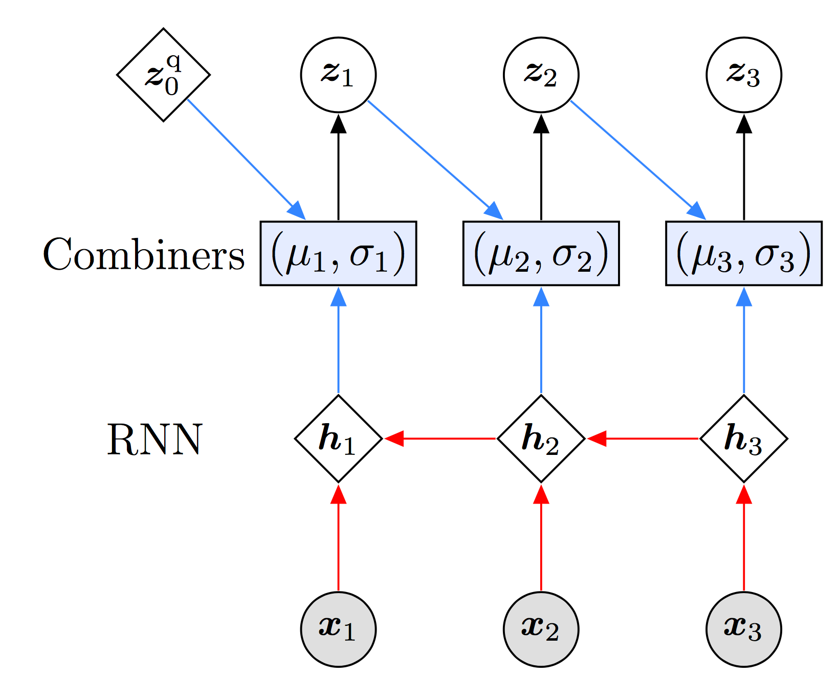
At the bottom of the figure we have our sequence of three observations. These observations will be consumed by a RNN that reads the observations from right to left and outputs three hidden states \(\{ {\bf h}_1, {\bf h}_2,{\bf h}_3\}\). Note that this computation is done before we sample any latent variables. Next, each of the hidden states will be fed into a Combiner module whose job is to output the mean and covariance of the the conditional distribution
\(q({\bf z}_t | {\bf z}_{t-1}, {\bf x}_{t:T})\), which we take to be given by a diagonal gaussian distribution. (Just like in the model, the conditional structure of \({\bf z}_{1:T}\) in the guide is such that we sample \({\bf z}_t\) forward in time.) In addition to the RNN hidden state, the Combiner also takes the latent random variable from the previous time step as input, except for \(t=1\), where it instead takes the trainable (variational) parameter
\({\bf z}_0^{\rm{q}}\).
Aside: Guide Structure
Why do we setup the RNN to consume the observations from right to left? Why not left to right? With this choice our conditional distribution \(q({\bf z}_t |...)\) depends on two things:
the latent \({\bf z}_{t-1}\) from the previous time step; and
the observations \({\bf x}_{t:T}\), i.e. the current observation together with all future observations
We are free to make other choices; all that is required is that that the guide is a properly normalized distribution that plays nice with autograd. This particular choice is motivated by the dependency structure of the true posterior: see reference [1] for a detailed discussion. In brief, while we could, for example, condition on the entire sequence of observations, because of the markov structure of the model everything that we need to know about the previous observations \({\bf x}_{1:t-1}\) is encapsulated by \({\bf z}_{t-1}\). We could condition on more things, but there’s no need; and doing so will probably tend to dilute the learning signal. So running the RNN from right to left is the most natural choice for this particular model.
Let’s look at the component parts in detail. First, the Combiner module:
class Combiner(nn.Module):
    """
    Parameterizes q(z_t | z_{t-1}, x_{t:T}), which is the basic building block
    of the guide (i.e. the variational distribution). The dependence on x_{t:T} is
    through the hidden state of the RNN (see the pytorch module `rnn` below)
    """
    def __init__(self, z_dim, rnn_dim):
        super().__init__()
        # initialize the three linear transformations used in the neural network
        self.lin_z_to_hidden = nn.Linear(z_dim, rnn_dim)
        self.lin_hidden_to_loc = nn.Linear(rnn_dim, z_dim)
        self.lin_hidden_to_scale = nn.Linear(rnn_dim, z_dim)
        # initialize the two non-linearities used in the neural network
        self.tanh = nn.Tanh()
        self.softplus = nn.Softplus()

    def forward(self, z_t_1, h_rnn):
        """
        Given the latent z at at a particular time step t-1 as well as the hidden
        state of the RNN h(x_{t:T}) we return the mean and scale vectors that
        parameterize the (diagonal) gaussian distribution q(z_t | z_{t-1}, x_{t:T})
        """
        # combine the rnn hidden state with a transformed version of z_t_1
        h_combined = 0.5 * (self.tanh(self.lin_z_to_hidden(z_t_1)) + h_rnn)
        # use the combined hidden state to compute the mean used to sample z_t
        loc = self.lin_hidden_to_loc(h_combined)
        # use the combined hidden state to compute the scale used to sample z_t
        scale = self.softplus(self.lin_hidden_to_scale(h_combined))
        # return loc, scale which can be fed into Normal
        return loc, scale
This module has the same general structure as Emitter and GatedTransition in the model. The only thing of note is that because the Combiner needs to consume two inputs at each time step, it transforms the inputs into a single combined hidden state h_combined before it computes the outputs.
Apart from the RNN, we now have all the ingredients we need to construct our guide distribution. Happily, PyTorch has great built-in RNN modules, so we don’t have much work to do here. We’ll see where we instantiate the RNN later. Let’s instead jump right into the definition of the stochastic function guide().
def guide(self, mini_batch, mini_batch_reversed, mini_batch_mask,
          mini_batch_seq_lengths, annealing_factor=1.0):

    # this is the number of time steps we need to process in the mini-batch
    T_max = mini_batch.size(1)
    # register all PyTorch (sub)modules with pyro
    pyro.module("dmm", self)

    # if on gpu we need the fully broadcast view of the rnn initial state
    # to be in contiguous gpu memory
    h_0_contig = self.h_0.expand(1, mini_batch.size(0),
                                 self.rnn.hidden_size).contiguous()
    # push the observed x's through the rnn;
    # rnn_output contains the hidden state at each time step
    rnn_output, _ = self.rnn(mini_batch_reversed, h_0_contig)
    # reverse the time-ordering in the hidden state and un-pack it
    rnn_output = poly.pad_and_reverse(rnn_output, mini_batch_seq_lengths)
    # set z_prev = z_q_0 to setup the recursive conditioning in q(z_t |...)
    z_prev = self.z_q_0.expand(mini_batch.size(0), self.z_q_0.size(0))

    # we enclose all the sample statements in the guide in a plate.
    # this marks that each datapoint is conditionally independent of the others.
    with pyro.plate("z_minibatch", len(mini_batch)):
        # sample the latents z one time step at a time
        for t in range(1, T_max + 1):
            # the next two lines assemble the distribution q(z_t | z_{t-1}, x_{t:T})
            z_loc, z_scale = self.combiner(z_prev, rnn_output[:, t - 1, :])
            z_dist = dist.Normal(z_loc, z_scale)

            # sample z_t from the distribution z_dist
            with pyro.poutine.scale(None, annealing_factor):
                z_t = pyro.sample("z_%d" % t,
                                  z_dist.mask(mini_batch_mask[:, t - 1:t])
                                        .to_event(1))
            # the latent sampled at this time step will be conditioned
            # upon in the next time step so keep track of it
            z_prev = z_t
The high-level structure of guide() is very similar to model(). First note that the model and guide take the same arguments: this is a general requirement for model/guide pairs in Pyro. As in the model, there’s a call to pyro.module that registers all the parameters with Pyro. Also, the for loop has the same structure as the one in model(), with the difference that the guide only needs to sample latents (there are no sample statements with the obs keyword). Finally,
note that the names of the latent variables in the guide exactly match those in the model. This is how Pyro knows to correctly align random variables.
The RNN logic should be familar to PyTorch users, but let’s go through it quickly. First we prepare the initial state of the RNN, h_0. Then we invoke the RNN via its forward call; the resulting tensor rnn_output contains the hidden states for the entire mini-batch. Note that because we want the RNN to consume the observations from right to left, the input to the RNN is mini_batch_reversed, which is a copy of mini_batch with all the sequences running in reverse temporal order.
Furthermore, mini_batch_reversed has been wrapped in a PyTorch rnn.pack_padded_sequence so that the RNN can deal with variable-length sequences. Since we do our sampling in latent space in normal temporal order, we use the helper function pad_and_reverse to reverse the hidden state sequences in rnn_output, so that we can feed the Combiner RNN hidden states that are correctly aligned and ordered. This helper function also unpacks the rnn_output so that it is no longer in
the form of a PyTorch rnn.pack_padded_sequence.
Packaging the Model and Guide as a PyTorch Module
At this juncture, we’re ready to proceed to inference. But before we do so let’s quickly go over how we packaged the model and guide as a single PyTorch Module. This is generally good practice, especially for larger models.
class DMM(nn.Module):
    """
    This PyTorch Module encapsulates the model as well as the
    variational distribution (the guide) for the Deep Markov Model
    """
    def __init__(self, input_dim=88, z_dim=100, emission_dim=100,
                 transition_dim=200, rnn_dim=600, rnn_dropout_rate=0.0,
                 num_iafs=0, iaf_dim=50, use_cuda=False):
        super().__init__()
        # instantiate pytorch modules used in the model and guide below
        self.emitter = Emitter(input_dim, z_dim, emission_dim)
        self.trans = GatedTransition(z_dim, transition_dim)
        self.combiner = Combiner(z_dim, rnn_dim)
        self.rnn = nn.RNN(input_size=input_dim, hidden_size=rnn_dim,
                          nonlinearity='relu', batch_first=True,
                          bidirectional=False, num_layers=1, dropout=rnn_dropout_rate)

        # define a (trainable) parameters z_0 and z_q_0 that help define
        # the probability distributions p(z_1) and q(z_1)
        # (since for t = 1 there are no previous latents to condition on)
        self.z_0 = nn.Parameter(torch.zeros(z_dim))
        self.z_q_0 = nn.Parameter(torch.zeros(z_dim))
        # define a (trainable) parameter for the initial hidden state of the rnn
        self.h_0 = nn.Parameter(torch.zeros(1, 1, rnn_dim))

        self.use_cuda = use_cuda
        # if on gpu cuda-ize all pytorch (sub)modules
        if use_cuda:
            self.cuda()

    # the model p(x_{1:T} | z_{1:T}) p(z_{1:T})
    def model(...):

        # ... as above ...

    # the guide q(z_{1:T} | x_{1:T}) (i.e. the variational distribution)
    def guide(...):

        # ... as above ...
Since we’ve already gone over model and guide, our focus here is on the constructor. First we instantiate the four PyTorch modules that we use in our model and guide. On the model-side: Emitter and GatedTransition. On the guide-side: Combiner and the RNN.
Next we define PyTorch Parameters for the initial state of the RNN as well as z_0 and z_q_0, which are fed into self.trans and self.combiner, respectively, in lieu of the non-existent random variable \(\bf z_0\).
The important point to make here is that all of these Modules and Parameters are attributes of DMM (which itself inherits from nn.Module). This has the consequence they are all automatically registered as belonging to the module. So, for example, when we call parameters() on an instance of DMM, PyTorch will know to return all the relevant parameters. It also means that when we invoke pyro.module("dmm", self) in model() and guide(), all the parameters of
both the model and guide will be registered with Pyro. Finally, it means that if we’re running on a GPU, the call to cuda() will move all the parameters into GPU memory.
Stochastic Variational Inference
With our model and guide at hand, we’re finally ready to do inference. Before we look at the full logic that is involved in a complete experimental script, let’s first see how to take a single gradient step. First we instantiate an instance of DMM and setup an optimizer.
# instantiate the dmm
dmm = DMM(input_dim, z_dim, emission_dim, transition_dim, rnn_dim,
          args.rnn_dropout_rate, args.num_iafs, args.iaf_dim, args.cuda)

# setup optimizer
adam_params = {"lr": args.learning_rate, "betas": (args.beta1, args.beta2),
               "clip_norm": args.clip_norm, "lrd": args.lr_decay,
               "weight_decay": args.weight_decay}
optimizer = ClippedAdam(adam_params)
Here we’re using an implementation of the Adam optimizer that includes gradient clipping. This mitigates some of the problems that can occur when training recurrent neural networks (e.g. vanishing/exploding gradients). Next we setup the inference algorithm.
# setup inference algorithm
svi = SVI(dmm.model, dmm.guide, optimizer, Trace_ELBO())
The inference algorithm SVI uses a stochastic gradient estimator to take gradient steps on an objective function, which in this case is given by the ELBO (the evidence lower bound). As the name indicates, the ELBO is a lower bound to the log evidence: \(\log p(\mathcal{D})\). As we take gradient steps that maximize the ELBO, we move our guide \(q(\cdot)\) closer to the exact posterior.
The argument Trace_ELBO() constructs a version of the gradient estimator that doesn’t need access to the dependency structure of the model and guide. Since all the latent variables in our model are reparameterizable, this is the appropriate gradient estimator for our use case. (It’s also the default option.)
Assuming we’ve prepared the various arguments of dmm.model and dmm.guide, taking a gradient step is accomplished by calling
svi.step(mini_batch, ...)
That’s all there is to it!
Well, not quite. This will be the main step in our inference algorithm, but we still need to implement a complete training loop with preparation of mini-batches, evaluation, and so on. This sort of logic will be familiar to any deep learner but let’s see how it looks in PyTorch/Pyro.
The Black Magic of Optimization
Actually, before we get to the guts of training, let’s take a moment and think a bit about the optimization problem we’ve setup. We’ve traded Bayesian inference in a non-linear model with a high-dimensional latent space—a hard problem—for a particular optimization problem. Let’s not kid ourselves, this optimization problem is pretty hard too. Why? Let’s go through some of the reasons:
the space of parameters we’re optimizing over is very high-dimensional (it includes all the weights in all the neural networks we’ve defined).
our objective function (the ELBO) cannot be computed analytically. so our parameter updates will be following noisy Monte Carlo gradient estimates
data-subsampling serves as an additional source of stochasticity: even if we wanted to, we couldn’t in general take gradient steps on the ELBO defined over the whole dataset (actually in our particular case the dataset isn’t so large, but let’s ignore that).
given all the neural networks and non-linearities we have in the loop, our (stochastic) loss surface is highly non-trivial
The upshot is that if we’re going to find reasonable (local) optima of the ELBO, we better take some care in deciding how to do optimization. This isn’t the time or place to discuss all the different strategies that one might adopt, but it’s important to emphasize how decisive a good or bad choice in learning hyperparameters (the learning rate, the mini-batch size, etc.) can be.
Before we move on, let’s discuss one particular optimization strategy that we’re making use of in greater detail: KL annealing. In our case the ELBO is the sum of two terms: an expected log likelihood term (which measures model fit) and a sum of KL divergence terms (which serve to regularize the approximate posterior):
\(\rm{ELBO} = \mathbb{E}_{q({\bf z}_{1:T})}[\log p({\bf x}_{1:T}|{\bf z}_{1:T})] - \mathbb{E}_{q({\bf z}_{1:T})}[ \log q({\bf z}_{1:T}) - \log p({\bf z}_{1:T})]\)
This latter term can be a quite strong regularizer, and in early stages of training it has a tendency to favor regions of the loss surface that contain lots of bad local optima. One strategy to avoid these bad local optima, which was also adopted in reference [1], is to anneal the KL divergence terms by multiplying them by a scalar annealing_factor that ranges between zero and one:
\(\mathbb{E}_{q({\bf z}_{1:T})}[\log p({\bf x}_{1:T}|{\bf z}_{1:T})] - \rm{annealing\_factor} \times \mathbb{E}_{q({\bf z}_{1:T})}[ \log q({\bf z}_{1:T}) - \log p({\bf z}_{1:T})]\)
The idea is that during the course of training the annealing_factor rises slowly from its initial value at/near zero to its final value at 1.0. The annealing schedule is arbitrary; below we will use a simple linear schedule. In terms of code, to scale the log likelihoods by the appropriate annealing factor we enclose each of the latent sample statements in the model and guide with a pyro.poutine.scale context.
Finally, we should mention that the main difference between the DMM implementation described here and the one used in reference [1] is that they take advantage of the analytic formula for the KL divergence between two gaussian distributions (whereas we rely on Monte Carlo estimates). This leads to lower variance gradient estimates of the ELBO, which makes training a bit easier. We can still train the model without making this analytic substitution, but training probably takes somewhat longer because of the higher variance. To use analytic KL divergences use TraceMeanField_ELBO.
Data Loading, Training, and Evaluation
First we load the data. There are 229 sequences in the training dataset, each with an average length of ~60 time steps.
jsb_file_loc = "./data/jsb_processed.pkl"
data = pickle.load(open(jsb_file_loc, "rb"))
training_seq_lengths = data['train']['sequence_lengths']
training_data_sequences = data['train']['sequences']
test_seq_lengths = data['test']['sequence_lengths']
test_data_sequences = data['test']['sequences']
val_seq_lengths = data['valid']['sequence_lengths']
val_data_sequences = data['valid']['sequences']
N_train_data = len(training_seq_lengths)
N_train_time_slices = np.sum(training_seq_lengths)
N_mini_batches = int(N_train_data / args.mini_batch_size +
                     int(N_train_data % args.mini_batch_size > 0))
For this dataset we will typically use a mini_batch_size of 20, so that there will be 12 mini-batches per epoch. Next we define the function process_minibatch which prepares a mini-batch for training and takes a gradient step:
def process_minibatch(epoch, which_mini_batch, shuffled_indices):
    if args.annealing_epochs > 0 and epoch < args.annealing_epochs:
        # compute the KL annealing factor appropriate
        # for the current mini-batch in the current epoch
        min_af = args.minimum_annealing_factor
        annealing_factor = min_af + (1.0 - min_af) * \
            (float(which_mini_batch + epoch * N_mini_batches + 1) /
             float(args.annealing_epochs * N_mini_batches))
    else:
        # by default the KL annealing factor is unity
        annealing_factor = 1.0

    # compute which sequences in the training set we should grab
    mini_batch_start = (which_mini_batch * args.mini_batch_size)
    mini_batch_end = np.min([(which_mini_batch + 1) * args.mini_batch_size,
                             N_train_data])
    mini_batch_indices = shuffled_indices[mini_batch_start:mini_batch_end]
    # grab the fully prepped mini-batch using the helper function in the data loader
    mini_batch, mini_batch_reversed, mini_batch_mask, mini_batch_seq_lengths \
        = poly.get_mini_batch(mini_batch_indices, training_data_sequences,
                              training_seq_lengths, cuda=args.cuda)
    # do an actual gradient step
    loss = svi.step(mini_batch, mini_batch_reversed, mini_batch_mask,
                     mini_batch_seq_lengths, annealing_factor)
    # keep track of the training loss
    return loss
We first compute the KL annealing factor appropriate to the mini-batch (according to a linear schedule as described earlier). We then compute the mini-batch indices, which we pass to the helper function get_mini_batch. This helper function takes care of a number of different things:
it sorts each mini-batch by sequence length
it calls another helper function to get a copy of the mini-batch in reversed temporal order
it packs each reversed mini-batch in a
rnn.pack_padded_sequence, which is then ready to be ingested by the RNNit cuda-izes all tensors if we’re on a GPU
it calls another helper function to get an appropriate 0/1 mask for the mini-batch
We then pipe all the return values of get_mini_batch() into elbo.step(...). Recall that these arguments will be further piped to model(...) and guide(...) during construction of the gradient estimator in elbo. Finally, we return a float which is a noisy estimate of the loss for that mini-batch.
We now have all the ingredients required for the main bit of our training loop:
times = [time.time()]
for epoch in range(args.num_epochs):
    # accumulator for our estimate of the negative log likelihood
    # (or rather -elbo) for this epoch
    epoch_nll = 0.0
    # prepare mini-batch subsampling indices for this epoch
    shuffled_indices = np.arange(N_train_data)
    np.random.shuffle(shuffled_indices)

    # process each mini-batch; this is where we take gradient steps
    for which_mini_batch in range(N_mini_batches):
        epoch_nll += process_minibatch(epoch, which_mini_batch, shuffled_indices)

    # report training diagnostics
    times.append(time.time())
    epoch_time = times[-1] - times[-2]
    log("[training epoch %04d]  %.4f \t\t\t\t(dt = %.3f sec)" %
        (epoch, epoch_nll / N_train_time_slices, epoch_time))
At the beginning of each epoch we shuffle the indices pointing to the training data. We then process each mini-batch until we’ve gone through the entire training set, accumulating the training loss as we go. Finally we report some diagnostic info. Note that we normalize the loss by the total number of time slices in the training set (this allows us to compare to reference [1]).
Evaluation
This training loop is still missing any kind of evaluation diagnostics. Let’s fix that. First we need to prepare the validation and test data for evaluation. Since the validation and test datasets are small enough that we can easily fit them into memory, we’re going to process each dataset batchwise (i.e. we will not be breaking up the dataset into mini-batches). [Aside: at this point the reader may ask why we don’t do the same thing for the training set. The reason is that additional stochasticity due to data-subsampling is often advantageous during optimization: in particular it can help us avoid local optima.] And, in fact, in order to get a lessy noisy estimate of the ELBO, we’re going to compute a multi-sample estimate. The simplest way to do this would be as follows:
val_loss = svi.evaluate_loss(val_batch, ..., num_particles=5)
This, however, would involve an explicit for loop with five iterations. For our particular model, we can do better and vectorize the whole computation. The only way to do this currently in Pyro is to explicitly replicate the data n_eval_samples many times. This is the strategy we follow:
# package repeated copies of val/test data for faster evaluation
# (i.e. set us up for vectorization)
def rep(x):
    return np.repeat(x, n_eval_samples, axis=0)

# get the validation/test data ready for the dmm: pack into sequences, etc.
val_seq_lengths = rep(val_seq_lengths)
test_seq_lengths = rep(test_seq_lengths)
val_batch, val_batch_reversed, val_batch_mask, val_seq_lengths = poly.get_mini_batch(
    np.arange(n_eval_samples * val_data_sequences.shape[0]), rep(val_data_sequences),
    val_seq_lengths, cuda=args.cuda)
test_batch, test_batch_reversed, test_batch_mask, test_seq_lengths = \
    poly.get_mini_batch(np.arange(n_eval_samples * test_data_sequences.shape[0]),
                        rep(test_data_sequences),
                        test_seq_lengths, cuda=args.cuda)
With the test and validation data now fully prepped, we define the helper function that does the evaluation:
def do_evaluation():
    # put the RNN into evaluation mode (i.e. turn off drop-out if applicable)
    dmm.rnn.eval()

    # compute the validation and test loss
    val_nll = svi.evaluate_loss(val_batch, val_batch_reversed, val_batch_mask,
                                 val_seq_lengths) / np.sum(val_seq_lengths)
    test_nll = svi.evaluate_loss(test_batch, test_batch_reversed, test_batch_mask,
                                  test_seq_lengths) / np.sum(test_seq_lengths)

    # put the RNN back into training mode (i.e. turn on drop-out if applicable)
    dmm.rnn.train()
    return val_nll, test_nll
We simply call the evaluate_loss method of elbo, which takes the same arguments as step(), namely the arguments that are passed to the model and guide. Note that we have to put the RNN into and out of evaluation mode to account for dropout. We can now stick do_evaluation() into the training loop; see the source code for details.
Results
Let’s make sure that our implementation gives reasonable results. We can use the numbers reported in reference [1] as a sanity check. For the same dataset and a similar model/guide setup (dimension of the latent space, number of hidden units in the RNN, etc.) they report a normalized negative log likelihood (NLL) of 6.93 on the testset (lower is better\()^{\S}\). This is to be compared to our result of 6.87. These numbers are very much in the same ball park, which is reassuring. It
seems that, at least for this dataset, not using analytic expressions for the KL divergences doesn’t degrade the quality of the learned model (although, as discussed above, the training probably takes somewhat longer).
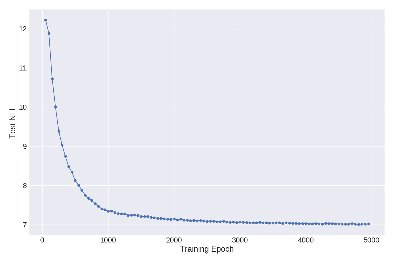
In the figure we show how the test NLL progresses during training for a single sample run (one with a rather conservative learning rate). Most of the progress is during the first 3000 epochs or so, with some marginal gains if we let training go on for longer. On a GeForce GTX 1080, 5000 epochs takes about 20 hours.
|
test NLL |
|---|---|
|
|
|
|
|
|
Finally, we also report results for guides with normalizing flows in the mix (details to be found in the next section).
\({ \S\;}\) Actually, they seem to report two numbers—6.93 and 7.03—for the same model/guide and it’s not entirely clear how the two reported numbers are different.
Bells, whistles, and other improvements
Inverse Autoregressive Flows
One of the great things about a probabilistic programming language is that it encourages modularity. Let’s showcase an example in the context of the DMM. We’re going to make our variational distribution richer by adding normalizing flows to the mix (see reference [2] for a discussion). This will only cost us four additional lines of code!
First, in the DMM constructor we add
iafs = [AffineAutoregressive(AutoRegressiveNN(z_dim, [iaf_dim])) for _ in range(num_iafs)]
self.iafs = nn.ModuleList(iafs)
This instantiates num_iafs many bijective transforms of the AffineAutoregressive type (see references [3,4]); each normalizing flow will have iaf_dim many hidden units. We then bundle the normalizing flows in a nn.ModuleList; this is just the PyTorchy way to package a list of nn.Modules. Next, in the guide we add the lines
if self.iafs.__len__() > 0:
    z_dist = TransformedDistribution(z_dist, self.iafs)
Here we’re taking the base distribution z_dist, which in our case is a conditional gaussian distribution, and using the TransformedDistribution construct we transform it into a non-gaussian distribution that is, by construction, richer than the base distribution. Voila!
Checkpointing
If we want to recover from a catastrophic failure in our training loop, there are two kinds of state we need to keep track of. The first is the various parameters of the model and guide. The second is the state of the optimizers (e.g. in Adam this will include the running average of recent gradient estimates for each parameter).
In Pyro, the parameters can all be found in the ParamStore. However, PyTorch also keeps track of them for us via the parameters() method of nn.Module. So one simple way we can save the parameters of the model and guide is to make use of the state_dict() method of dmm in conjunction with torch.save(); see below. In the case that we have AffineAutoregressive‘s in the loop, this is in fact the only option at our disposal. This is because the AffineAutoregressive
module contains what are called ’persistent buffers’ in PyTorch parlance. These are things that carry state but are not Parameters. The state_dict() and load_state_dict() methods of nn.Module know how to deal with buffers correctly.
To save the state of the optimizers, we have to use functionality inside of pyro.optim.PyroOptim. Recall that the typical user never interacts directly with PyTorch Optimizers when using Pyro; since parameters can be created dynamically in an arbitrary probabilistic program, Pyro needs to manage Optimizers for us. In our case saving the optimizer state will be as easy as calling optimizer.save(). The loading logic is entirely analagous. So our entire logic for saving and loading
checkpoints only takes a few lines:
# saves the model and optimizer states to disk
def save_checkpoint():
    log("saving model to %s..." % args.save_model)
    torch.save(dmm.state_dict(), args.save_model)
    log("saving optimizer states to %s..." % args.save_opt)
    optimizer.save(args.save_opt)
    log("done saving model and optimizer checkpoints to disk.")

# loads the model and optimizer states from disk
def load_checkpoint():
    assert exists(args.load_opt) and exists(args.load_model), \
        "--load-model and/or --load-opt misspecified"
    log("loading model from %s..." % args.load_model)
    dmm.load_state_dict(torch.load(args.load_model))
    log("loading optimizer states from %s..." % args.load_opt)
    optimizer.load(args.load_opt)
    log("done loading model and optimizer states.")
Some final comments
A deep markov model is a relatively complex model. Now that we’ve taken the effort to implement a version of the deep markov model tailored to the polyphonic music dataset, we should ask ourselves what else we can do. What if we’re handed a different sequential dataset? Do we have to start all over?
Not at all! The beauty of probalistic programming is that it enables—and encourages—modular approaches to modeling and inference. Adapting our polyphonic music model to a dataset with continuous observations is as simple as changing the observation likelihood. The vast majority of the code could be taken over unchanged. This means that with a little bit of extra work, the code in this tutorial could be repurposed to enable a huge variety of different models.
See the complete code on Github.
References
[1] Structured Inference Networks for Nonlinear State Space Models, Rahul G. Krishnan, Uri Shalit, David Sontag
[2] Variational Inference with Normalizing Flows, Danilo Jimenez Rezende, Shakir Mohamed
[3] Improving Variational Inference with Inverse Autoregressive Flow, Diederik P. Kingma, Tim Salimans, Rafal Jozefowicz, Xi Chen, Ilya Sutskever, Max Welling
[4] MADE: Masked Autoencoder for Distribution Estimation, Mathieu Germain, Karol Gregor, Iain Murray, Hugo Larochelle
[5] Modeling Temporal Dependencies in High-Dimensional Sequences: Application to Polyphonic Music Generation and Transcription, Boulanger-Lewandowski, N., Bengio, Y. and Vincent, P.