Designing Adaptive Experiments to Study Working Memory¶

In most of machine learning, we begin with data and go on to learn a model. In other contexts, we also have a hand in the data generation process. This gives us an exciting opportunity: we can try to obtain data that will help our model learn more effectively. This procedure is called optimal experimental design (OED) and Pyro supports choosing optimal designs through the pyro.contrib.oed module.

When using OED, the data generation and modelling works as follows:

Write down a Bayesian model involving a design parameter, an unknown latent variable and an observable.
Choose the optimal design (more details on this later).
Collect the data and fit the model, e.g. using SVI.

We can also run multiple ‘rounds’ or iterations of experiments. When doing this, we take the learned model from step 3 and use it as our prior in step 1 for the next round. This approach can be particularly useful because it allows us to design the next experiment based on what has already been learned: the experiments are adaptive.

In this tutorial, we work through a specific example of this entire OED procedure with multiple rounds. We will show how to design adaptive experiments to learn a participant’s working memory capacity. The design we will be adapting is the length of a sequence of digits that we ask a participant to remember. Let’s dive into the full details.

The experiment set-up¶

Suppose you, the participant, are shown a sequence of digits

\[1\ 4\ 7\ 0\ 9\]

which are then hidden. You have to to reproduce the sequence exactly from memory. In the next round, the length of the sequence may be different

\[6\ 5\ 0\ 2\ 8\ 0 .\]

The longest sequence that you can remember is your working memory capacity. In this tutorial, we build a Bayesian model for working memory, and use it to run an adaptive sequence of experiments that very quickly learn someone’s working memory capacity.

A model of working memory¶

Our model for a single round of the digits experiment described above has three components: the length \(l\) of the sequence that the participant has to remember, the participant’s true working memory capacity \(\theta\), and the outcome of the experiment \(y\) which indicates whether they were able to remember the sequence successfully (\(y=1\)) or not (\(y=0\)). We choose a prior for working memory capacity based on the (in)famous “The magical number seven, plus or minus two” [1].

Note: \(\theta\) actually represents the point where the participant has a 50/50 chance of remembering the sequence correctly.

[2]:

import torch

import pyro
import pyro.distributions as dist


sensitivity = 1.0
prior_mean = torch.tensor(7.0)
prior_sd = torch.tensor(2.0)


def model(l):
    # Dimension -1 of `l` represents the number of rounds
    # Other dimensions are batch dimensions: we indicate this with a plate_stack
    with pyro.plate_stack("plate", l.shape[:-1]):
        theta = pyro.sample("theta", dist.Normal(prior_mean, prior_sd))
        # Share theta across the number of rounds of the experiment
        # This represents repeatedly testing the same participant
        theta = theta.unsqueeze(-1)
        # This define a *logistic regression* model for y
        logit_p = sensitivity * (theta - l)
        # The event shape represents responses from the same participant
        y = pyro.sample("y", dist.Bernoulli(logits=logit_p).to_event(1))
        return y

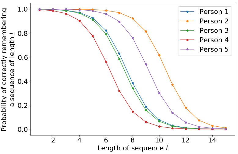
The probability of successfully remembering the sequence is plotted below, for five random samples of \(\theta\).

[4]:

import matplotlib
import matplotlib.pyplot as plt

matplotlib.rcParams.update({'font.size': 22})

# We sample five times from the prior
theta = (prior_mean + prior_sd * torch.randn((5,1)))
l = torch.arange(1, 16, dtype=torch.float)
# This is the same as using 'logits=' in the prior above
prob = torch.sigmoid(sensitivity * (theta - l))

plt.figure(figsize=(12, 8))
for curve in torch.unbind(prob, 0):
    plt.plot(l.numpy(), curve.numpy(), marker='o')
plt.xlabel("Length of sequence $l$")
plt.ylabel("Probability of correctly remembering\na sequence of length $l$")
plt.legend(["Person {}".format(i+1) for i in range(5)])
plt.show()

Inference in the model¶

With the model in hand, we quickly demonstrate variational inference in Pyro for this model. We define a Normal guide for variational inference.

[5]:

from torch.distributions.constraints import positive

def guide(l):
    # The guide is initialised at the prior
    posterior_mean = pyro.param("posterior_mean", prior_mean.clone())
    posterior_sd = pyro.param("posterior_sd", prior_sd.clone(), constraint=positive)
    pyro.sample("theta", dist.Normal(posterior_mean, posterior_sd))

We finally specify the following data: the participant was shown sequences of lengths 5, 7 and 9. They remembered the first two correctly, but not the third one.

[6]:

l_data = torch.tensor([5., 7., 9.])
y_data = torch.tensor([1., 1., 0.])

We can now run SVI on the model.

[7]:

from pyro.infer import SVI, Trace_ELBO
from pyro.optim import Adam

conditioned_model = pyro.condition(model, {"y": y_data})
svi = SVI(conditioned_model,
          guide,
          Adam({"lr": .001}),
          loss=Trace_ELBO(),
          num_samples=100)
pyro.clear_param_store()
num_iters = 5000
for i in range(num_iters):
    elbo = svi.step(l_data)
    if i % 500 == 0:
        print("Neg ELBO:", elbo)

Neg ELBO: 1.6167092323303223
Neg ELBO: 3.706324815750122
Neg ELBO: 0.9958380460739136
Neg ELBO: 1.0630500316619873
Neg ELBO: 1.1738307476043701
Neg ELBO: 1.6654635667800903
Neg ELBO: 1.296904444694519
Neg ELBO: 1.305729627609253
Neg ELBO: 1.2626266479492188
Neg ELBO: 1.3095542192459106

[9]:

print("Prior:     N({:.3f}, {:.3f})".format(prior_mean, prior_sd))
print("Posterior: N({:.3f}, {:.3f})".format(pyro.param("posterior_mean"),
                                            pyro.param("posterior_sd")))

Prior:     N(7.000, 2.000)
Posterior: N(7.749, 1.282)

Under our posterior, we can see that we have an updated estimate for the participant’s working memory capacity, and our uncertainty has now decreased.

Bayesian optimal experimental design¶

So far so standard. In the previous example, the lengths l_data were not chosen with a great deal of forethought. Fortunately, in a setting like this, it is possible to use a more sophisticated strategy to choose the sequence lengths to make the most of every question we ask.

We do this using Bayesian optimal experimental design (BOED). In BOED, we are interested in designing experiments that maximise the information gain, which is defined formally as

\[\text{IG}(l, y) = KL(p(\theta|y,l)||p(\theta)) .\]

where \(KL\) represents the Kullback-Leiber divergence.

In words, the information gain is the KL divergence from the posterior to the prior. It therefore represents the distance we “move” the posterior by running an experiment with length \(l\) and getting back the outcome \(y\).

Unfortunately, we will not know \(y\) until we actually run the experiment. Therefore, we choose \(l\) on the basis of the expected information gain [2]

\[\text{EIG}(l) = \mathbb{E}_{y\sim p(y|\theta,l)} [KL(p(\theta|y,l)||p(\theta))].\]

Because it features the posterior density \(p(y|\theta,l)\), the EIG is not immediately tractable. However, we can make use of the following variational estimator for EIG [3]

\[\text{EIG}(l) = \min_q \mathbb{E}_{\theta,y \sim p(\theta)p(y|\theta,l)} \left[ \log \frac{p(y|\theta,l)}{q(y|l)} \right].\]

Optimal experimental design in Pyro¶

Fortunately, Pyro comes ready with tools to estimate the EIG. All we have to do is define the “marginal guide” \(q(y|l)\) in the formula above.

[10]:

def marginal_guide(design, observation_labels, target_labels):
    # This shape allows us to learn a different parameter for each candidate design l
    q_logit = pyro.param("q_logit", torch.zeros(design.shape[-2:]))
    pyro.sample("y", dist.Bernoulli(logits=q_logit).to_event(1))

This is not a guide for inference, like the guides normally encountered in Pyro and used in SVI. Instead, this guide samples only the observed sample sites: in this case "y". This makes sense because conventional guides approximate the posterior \(p(\theta|y, l)\) whereas our guide approximates the marginal \(p(y|l)\).

[11]:

from pyro.contrib.oed.eig import marginal_eig

# The shape of `candidate_designs` is (number designs, 1)
# This represents a batch of candidate designs, each design is for one round of experiment
candidate_designs = torch.arange(1, 15, dtype=torch.float).unsqueeze(-1)
pyro.clear_param_store()
num_steps, start_lr, end_lr = 1000, 0.1, 0.001
optimizer = pyro.optim.ExponentialLR({'optimizer': torch.optim.Adam,
                                      'optim_args': {'lr': start_lr},
                                      'gamma': (end_lr / start_lr) ** (1 / num_steps)})

eig = marginal_eig(model,
                   candidate_designs,       # design, or in this case, tensor of possible designs
                   "y",                     # site label of observations, could be a list
                   "theta",                 # site label of 'targets' (latent variables), could also be list
                   num_samples=100,         # number of samples to draw per step in the expectation
                   num_steps=num_steps,     # number of gradient steps
                   guide=marginal_guide,    # guide q(y)
                   optim=optimizer,         # optimizer with learning rate decay
                   final_num_samples=10000  # at the last step, we draw more samples
                                            # for a more accurate EIG estimate
                  )

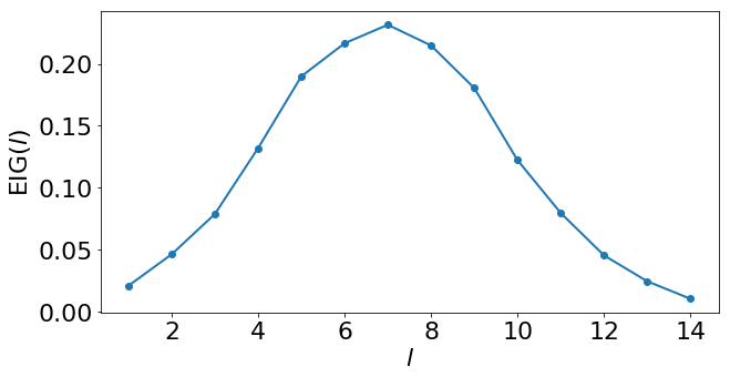
We can visualize the EIG estimates that we found.

[12]:

plt.figure(figsize=(10,5))
matplotlib.rcParams.update({'font.size': 22})
plt.plot(candidate_designs.numpy(), eig.detach().numpy(), marker='o', linewidth=2)
plt.xlabel("$l$")
plt.ylabel("EIG($l$)")
plt.show()

[13]:

best_l = 1 + torch.argmax(eig)
print("Optimal design:", best_l.item())

Optimal design: 7

This tells us that the first round should be run with a sequence of length 7. Note that, while we might have been able to guess this optimal design intuitively, this same framework applies equally well to more sophisticated models and experiments where finding the optimal design by intuition is more challenging.

As a side-effect of training, our marginal guide \(q(y|l)\) has approximately learned the marginal distribution \(p(y|l)\).

[14]:

q_prob = torch.sigmoid(pyro.param("q_logit"))
print("   l | q(y = 1 | l)")
for (l, q) in zip(candidate_designs, q_prob):
    print("{:>4} | {}".format(int(l.item()), q.item()))

   l | q(y = 1 | l)
   1 | 0.9849993586540222
   2 | 0.9676634669303894
   3 | 0.9329487681388855
   4 | 0.871809720993042
   5 | 0.7761920690536499
   6 | 0.6436398029327393
   7 | 0.4999988079071045
   8 | 0.34875917434692383
   9 | 0.22899287939071655
  10 | 0.13036076724529266
  11 | 0.06722454726696014
  12 | 0.03191758319735527
  13 | 0.015132307074964046
  14 | 0.00795808993279934

The elements of this fitted tensor represent the marginal over \(y\), for each possible sequence length \(l\) in candidate_designs. We have marginalised out the unknown \(\theta\) so this fitted tensor shows the probabilities for an ‘average’ participant.

The adaptive experiment¶

We now have the ingredients to build an adaptive experiment to study working memory. We repeat the following steps:

Use the EIG to find the optimal sequence length \(l\)
Run the test using a sequence of length \(l\)
Update the posterior distribution with the new data

At the first iteration, step 1 is done using the prior as above. However, for subsequent iterations, we use the posterior given all the data so far.

In this notebook, the “experiment” is performed using the following synthesiser

[15]:

def synthetic_person(l):
    # The synthetic person can remember any sequence shorter than 6
    # They cannot remember any sequence of length 6 or above
    # (There is no randomness in their responses)
    y = (l < 6.).float()
    return y

The following code allows us to update the model as we gather more data.

[16]:

def make_model(mean, sd):
    def model(l):
        # Dimension -1 of `l` represents the number of rounds
        # Other dimensions are batch dimensions: we indicate this with a plate_stack
        with pyro.plate_stack("plate", l.shape[:-1]):
            theta = pyro.sample("theta", dist.Normal(mean, sd))
            # Share theta across the number of rounds of the experiment
            # This represents repeatedly testing the same participant
            theta = theta.unsqueeze(-1)
            # This define a *logistic regression* model for y
            logit_p = sensitivity * (theta - l)
            # The event shape represents responses from the same participant
            y = pyro.sample("y", dist.Bernoulli(logits=logit_p).to_event(1))
            return y
    return model

Now we have everything to run a 10-step experiment using adaptive designs.

[17]:

ys = torch.tensor([])
ls = torch.tensor([])
history = [(prior_mean, prior_sd)]
pyro.clear_param_store()
current_model = make_model(prior_mean, prior_sd)

for experiment in range(10):
    print("Round", experiment + 1)

    # Step 1: compute the optimal length
    optimizer = pyro.optim.ExponentialLR({'optimizer': torch.optim.Adam,
                                          'optim_args': {'lr': start_lr},
                                          'gamma': (end_lr / start_lr) ** (1 / num_steps)})
    eig = marginal_eig(current_model, candidate_designs, "y", "theta", num_samples=100,
                       num_steps=num_steps, guide=marginal_guide, optim=optimizer,
                       final_num_samples=10000)
    best_l = 1 + torch.argmax(eig).float().detach()

    # Step 2: run the experiment, here using the synthetic person
    print("Asking the participant to remember a sequence of length", int(best_l.item()))
    y = synthetic_person(best_l)
    if y:
        print("Participant remembered correctly")
    else:
        print("Participant could not remember the sequence")
    # Store the sequence length and outcome
    ls = torch.cat([ls, best_l.expand(1)], dim=0)
    ys = torch.cat([ys, y.expand(1)])

    # Step 3: learn the posterior using all data seen so far
    conditioned_model = pyro.condition(model, {"y": ys})
    svi = SVI(conditioned_model,
              guide,
              Adam({"lr": .005}),
              loss=Trace_ELBO(),
              num_samples=100)
    num_iters = 2000
    for i in range(num_iters):
        elbo = svi.step(ls)

    history.append((pyro.param("posterior_mean").detach().clone().numpy(),
                    pyro.param("posterior_sd").detach().clone().numpy()))
    current_model = make_model(pyro.param("posterior_mean").detach().clone(),
                               pyro.param("posterior_sd").detach().clone())
    print("Estimate of \u03b8: {:.3f} \u00b1 {:.3f}\n".format(*history[-1]))

Round 1
Asking the participant to remember a sequence of length 7
Participant could not remember the sequence
Estimate of θ: 5.788 ± 1.636

Round 2
Asking the participant to remember a sequence of length 6
Participant could not remember the sequence
Estimate of θ: 4.943 ± 1.252

Round 3
Asking the participant to remember a sequence of length 5
Participant remembered correctly
Estimate of θ: 5.731 ± 1.043

Round 4
Asking the participant to remember a sequence of length 6
Participant could not remember the sequence
Estimate of θ: 5.261 ± 0.928

Round 5
Asking the participant to remember a sequence of length 5
Participant remembered correctly
Estimate of θ: 5.615 ± 0.859

Round 6
Asking the participant to remember a sequence of length 6
Participant could not remember the sequence
Estimate of θ: 5.423 ± 0.888

Round 7
Asking the participant to remember a sequence of length 6
Participant could not remember the sequence
Estimate of θ: 5.092 ± 0.763

Round 8
Asking the participant to remember a sequence of length 5
Participant remembered correctly
Estimate of θ: 5.371 ± 0.717

Round 9
Asking the participant to remember a sequence of length 5
Participant remembered correctly
Estimate of θ: 5.597 ± 0.720

Round 10
Asking the participant to remember a sequence of length 6
Participant could not remember the sequence
Estimate of θ: 5.434 ± 0.640

Now let’s visualize the evolution of the posterior over \(\theta\):

[19]:

import numpy as np
from scipy.stats import norm
import matplotlib.colors as colors
import matplotlib.cm as cmx


matplotlib.rcParams.update({'font.size': 22})
cmap = plt.get_cmap('winter')
cNorm  = colors.Normalize(vmin=0, vmax=len(history)-1)
scalarMap = cmx.ScalarMappable(norm=cNorm, cmap=cmap)
plt.figure(figsize=(12, 6))
x = np.linspace(0, 14, 100)
for idx, (mean, sd) in enumerate(history):
    color = scalarMap.to_rgba(idx)
    y = norm.pdf(x, mean, sd)
    plt.plot(x, y, color=color)
    plt.xlabel("$\\theta$")
    plt.ylabel("p.d.f.")
plt.show()

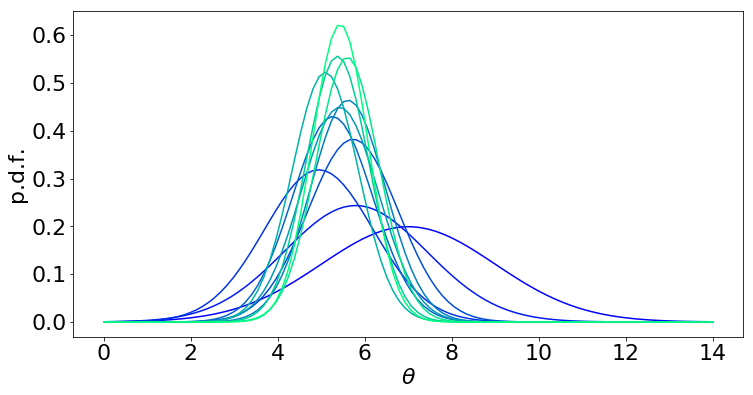
(Blue = prior, light green = 10 step posterior)

By contrast, suppose we use a simplistic design: try sequences of lengths 1, 2, …, 10.

[20]:

pyro.clear_param_store()
ls = torch.arange(1, 11, dtype=torch.float)
ys = synthetic_person(ls)
conditioned_model = pyro.condition(model, {"y": ys})
svi = SVI(conditioned_model,
          guide,
          Adam({"lr": .005}),
          loss=Trace_ELBO(),
          num_samples=100)
num_iters = 2000
for i in range(num_iters):
    elbo = svi.step(ls)

[22]:

plt.figure(figsize=(12,6))
matplotlib.rcParams.update({'font.size': 22})
y1 = norm.pdf(x, pyro.param("posterior_mean").detach().numpy(),
              pyro.param("posterior_sd").detach().numpy())
y2 = norm.pdf(x, history[-1][0], history[-1][1])
plt.plot(x, y1)
plt.plot(x, y2)
plt.legend(["Simple design", "Optimal design"])
plt.xlabel("$\\theta$")
plt.ylabel("p.d.f.")
plt.show()

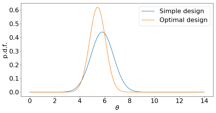
Although both design strategies give us data, the optimal strategy ends up with a posterior distribution that is more peaked: that means we have greater confidence in our final answer, or may be able to stop experimenting earlier.

Extensions¶

In this tutorial we used variational inference to fit an approximate posterior for \(\theta\). This could be substituted for an alternative posterior inference strategy, such as Hamiltonian Monte Carlo.

The model in this tutorial is very simple and could be extended in a number of ways. For instance, it’s possible that as well as measuring whether the participant did or did not remember the sequence, we might collect some other information as well. We could build a model for the number of mistakes made (e.g. the edit distance between the correct sequence and the participant’s response) or jointly model the correctness and the time taken to respond. Here is an example model where we model the response time using a LogNormal distribution, as suggested by [4].

[18]:

time_intercept = 0.5
time_scale = 0.5

def model(l):
    theta = pyro.sample("theta", dist.Normal(prior_mean, prior_sd))
    logit_p = sensitivity * (theta - l)
    correct = pyro.sample("correct", dist.Bernoulli(logits=logit_p))
    mean_log_time = time_intercept + time_scale * (theta - l)
    time = pyro.sample("time", dist.LogNormal(mean_log_time, 1.0))
    return correct, time

It would still be possible to compute the EIG using marginal_eig. We would replace "y" by ["correct", "time"] and the marginal guide would now model a joint distribution over the two sites "correct" and "time".

Our model also made a number of assumptions that we may choose to relax. For instance, we assumed that all sequences of the same length are equally easy to remember. We also fixed the sensitivity to be a known constant: it’s likely we would need to learn this. We could also think about learning at two levels: learning global variables for population trends as well as local variables for individual level effects. The current model is an individual only model. The EIG could still be used as a means to select the optimal design in such scenarios.

References¶

[1] Miller, G.A., 1956. The magical number seven, plus or minus two: Some limits on our capacity for processing information. Psychological review, 63(2), p.81.

[2] Chaloner, K. and Verdinelli, I., 1995. Bayesian experimental design: A review. Statistical Science, pp.273-304.

[3] Foster, A., Jankowiak, M., Bingham, E., Horsfall, P., Teh, Y.W., Rainforth, T. and Goodman, N., 2019. Variational Bayesian Optimal Experimental Design. Advances in Neural Information Processing Systems 2019 (to appear).

[4] van der Linden, W.J., 2006. A lognormal model for response times on test items. Journal of Educational and Behavioral Statistics, 31(2), pp.181-204.