High-dimensional Bayesian workflow, with applications to SARS-CoV-2 strains
This tutorial describes a workflow for incrementally building pipelines to analyze high-dimensional data in Pyro. This workflow has evolved over a few years of applying Pyro to models with \(10^5\) or more latent variables. We build on Gelman et al. (2020)’s concept of Bayesian workflow, and focus on aspects particular to high-dimensional models: approximate inference and numerical stability. While the individual components of the pipeline deserve their own tutorials, this tutorial focuses on incrementally combining those components.
The fastest way to find a good model of your data is to quickly discard many bad models, i.e. to iterate. In statistics we call this iterative workflow Box’s loop. An efficient workflow allows us to discard bad models as quickly as possible. Workflow efficiency demands that code changes to upstream components don’t break previous coding effort on downstream components. Pyro’s approaches to this challenge include strategies for variational approximations (pyro.infer.autoguide) and strategies for transforming model coordinate systems to improve geometry (pyro.infer.reparam).
Summary
Great models can only be achieved by iterative development.
Iterate quickly by building a pipeline that is robust to code changes.
Start with a simple model and mean-field inference.
Avoid NANs by intelligently initializing and .clamp()ing.
Reparametrize the model to improve geometry.
Create a custom variational family by combining AutoGuides or EasyGuides.
Table of contents
Overview
Consider the problem of sampling from the posterior distribution of a probabilistic model with \(10^5\) or more continuous latent variables, but whose data fits entirely in memory. (For larger datasets, consider amortized variational inference.) Inference in such high-dimensional models can be challenging even when posteriors are known to be unimodal or even log-concave, due to correlations among latent variables.
To perform inference in such high-dimensional models in Pyro, we have evolved a workflow to incrementally build data analysis pipelines combining variational inference, reparametrization effects, and ad-hoc initialization strategies. Our workflow is summarized as a sequence of steps, where validation after any step might suggest backtracking to change design decisions at a previous step.
Clean the data.
Create a generative model.
Sanity check using MAP or mean-field inference.
Create an initialization heuristic.
Reparameterize the model, evaluating results under mean field VI.
Customize the variational family (autoguides, easyguides, custom guides).
The crux of efficient workflow is to ensure changes don’t break your pipeline. That is, after you build a number of pipeline stages, validate results, and decide to change one component in the pipeline, you’d like to minimize code changes needed in other components. The remainder of this tutorial describes these steps individually, then describes nuances of interactions among stages, then provides an example.
Running example: SARS-CoV-2 strain prediction
The running example in this tutorial will be a model (Obermeyer et al. 2022) of the relative growth rates of different strains of the SARS-CoV-2 virus, based on open data counting different PANGO lineages of viral genomic samples collected at different times around the world. There are about 2 million sequences in total.
The model is a high-dimensional regression model with around 1000 coefficients, a multivariate logistic growth function (using a simple torch.softmax()) and a Multinomial likelihood. While the number of coefficients is relatively small, there are about 500,000 local latent variables to estimate, and plate structure in the model should lead to an approximately block diagonal posterior covariance matrix. For an introduction to simple logistic growth models using this same dataset, see the logistic growth tutorial.
[1]:
from collections import defaultdict
from pprint import pprint
import functools
import math
import os
import torch
import pyro
import pyro.distributions as dist
import pyro.poutine as poutine
from pyro.distributions import constraints
from pyro.infer import SVI, Trace_ELBO
from pyro.infer.autoguide import (
    AutoDelta,
    AutoNormal,
    AutoMultivariateNormal,
    AutoLowRankMultivariateNormal,
    AutoGuideList,
    init_to_feasible,
)
from pyro.infer.reparam import AutoReparam, LocScaleReparam
from pyro.nn.module import PyroParam
from pyro.optim import ClippedAdam
from pyro.ops.special import sparse_multinomial_likelihood
import matplotlib.pyplot as plt

if torch.cuda.is_available():
    print("Using GPU")
    torch.set_default_tensor_type("torch.cuda.FloatTensor")
else:
    print("Using CPU")
smoke_test = ('CI' in os.environ)
Using CPU
Clean the data
Our running example will use a pre-cleaned dataset. We started with Nextstrain’s ncov tool for preprocessing, followed by the Broad Institute’s pyro-cov tool for aggregation, resulting in a dataset of SARS-CoV-2 lineages observed around the world through time.
[2]:
from pyro.contrib.examples.nextstrain import load_nextstrain_counts
dataset = load_nextstrain_counts()

def summarize(x, name=""):
    if isinstance(x, dict):
        for k, v in sorted(x.items()):
            summarize(v, name + "." + k if name else k)
    elif isinstance(x, torch.Tensor):
        print(f"{name}: {type(x).__name__} of shape {tuple(x.shape)} on {x.device}")
    elif isinstance(x, list):
        print(f"{name}: {type(x).__name__} of length {len(x)}")
    else:
        print(f"{name}: {type(x).__name__}")
summarize(dataset)
counts: Tensor of shape (27, 202, 1316) on cpu
features: Tensor of shape (1316, 2634) on cpu
lineages: list of length 1316
locations: list of length 202
mutations: list of length 2634
sparse_counts.index: Tensor of shape (3, 57129) on cpu
sparse_counts.total: Tensor of shape (27, 202) on cpu
sparse_counts.value: Tensor of shape (57129,) on cpu
start_date: datetime
time_step_days: int
Create a generative model
The first step to using Pyro is creating a generative model, either a python function or a pyro.nn.Module. Start simple. Start with a shallow hierarchy and later add latent variables to share statistical strength. Start with a slice of your data then add a plate over multiple slices. Start with simple distributions like Normal, LogNormal, Poisson and Multinomial, then consider overdispersed versions like StudentT, Gamma, GammaPoisson/NegativeBinomial, and DirichletMultinomial. Keep your model simple and readable so you can share it and get feedback from domain experts. Use weakly informative priors.
We’ll focus on a multivariate logistic growth model of competing SARS-CoV-2 strains, as described in Obermeyer et al. (2022). This model uses a numerically stable logits parameter in its multinomial likelihood, rather than a probs parameter. Similarly upstream variables init, rate, rate_loc, and coef are all in log-space. This will mean e.g. that a zero coefficient has multiplicative effect of 1.0, and a
positive coefficient has multiplicative effect greater than 1.
Note we scale coef by 1/100 because we want to model a very small number, but the automatic parts of Pyro and PyTorch work best for numbers on the order of 1.0 rather than very small numbers. When we later interpret coef in a volcano plot we’ll need to duplicate this scaling factor.
[3]:
def model(dataset):
    features = dataset["features"]
    counts = dataset["counts"]
    assert features.shape[0] == counts.shape[-1]
    S, M = features.shape
    T, P, S = counts.shape
    time = torch.arange(float(T)) * dataset["time_step_days"] / 5.5
    time -= time.mean()
    strain_plate = pyro.plate("strain", S, dim=-1)
    place_plate = pyro.plate("place", P, dim=-2)
    time_plate = pyro.plate("time", T, dim=-3)

    # Model each region as multivariate logistic growth.
    rate_scale = pyro.sample("rate_scale", dist.LogNormal(-4, 2))
    init_scale = pyro.sample("init_scale", dist.LogNormal(0, 2))
    with pyro.plate("mutation", M, dim=-1):
        coef = pyro.sample("coef", dist.Laplace(0, 0.5))
    with strain_plate:
        rate_loc = pyro.deterministic("rate_loc", 0.01 * coef @ features.T)
    with place_plate, strain_plate:
        rate = pyro.sample("rate", dist.Normal(rate_loc, rate_scale))
        init = pyro.sample("init", dist.Normal(0, init_scale))
    logits = init + rate * time[:, None, None]

    # Observe sequences via a multinomial likelihood.
    with time_plate, place_plate:
        pyro.sample(
            "obs",
            dist.Multinomial(logits=logits.unsqueeze(-2), validate_args=False),
            obs=counts.unsqueeze(-2),
        )
The execution cost of this model is dominated by the multinomial likelihood over a large sparse count matrix.
[4]:
print("counts has {:d} / {} nonzero elements".format(
    dataset['counts'].count_nonzero(), dataset['counts'].numel()
))
counts has 57129 / 7177464 nonzero elements
To speed up inference (and model iteration!) we’ll replace the pyro.sample(..., Multinomial) likelihood with an equivalent but much cheaper pyro.factor statement using a helper pyro.ops.sparse_multinomial_likelihood.
[5]:
def model(dataset, predict=None):
    features = dataset["features"]
    counts = dataset["counts"]
    sparse_counts = dataset["sparse_counts"]
    assert features.shape[0] == counts.shape[-1]
    S, M = features.shape
    T, P, S = counts.shape
    time = torch.arange(float(T)) * dataset["time_step_days"] / 5.5
    time -= time.mean()

    # Model each region as multivariate logistic growth.
    rate_scale = pyro.sample("rate_scale", dist.LogNormal(-4, 2))
    init_scale = pyro.sample("init_scale", dist.LogNormal(0, 2))
    with pyro.plate("mutation", M, dim=-1):
        coef = pyro.sample("coef", dist.Laplace(0, 0.5))
    with pyro.plate("strain", S, dim=-1):
        rate_loc = pyro.deterministic("rate_loc", 0.01 * coef @ features.T)
        with pyro.plate("place", P, dim=-2):
            rate = pyro.sample("rate", dist.Normal(rate_loc, rate_scale))
            init = pyro.sample("init", dist.Normal(0, init_scale))
    if predict is not None:  # Exit early during evaluation.
        probs = (init + rate * time[predict]).softmax(-1)
        return probs
    logits = (init + rate * time[:, None, None]).log_softmax(-1)

    # Observe sequences via a cheap sparse multinomial likelihood.
    t, p, s = sparse_counts["index"]
    pyro.factor(
        "obs",
        sparse_multinomial_likelihood(
            sparse_counts["total"], logits[t, p, s], sparse_counts["value"]
        )
    )
Sanity check using mean field inference
Mean field Normal inference is cheap and robust, and is a good way to sanity check your posterior point estimate, even if the posterior uncertainty may be implausibly narrow. We recommend starting with an AutoNormal guide, and possibly setting init_scale to a small value like init_scale=0.01 or init_scale=0.001.
Note that while MAP estimating via AutoDelta is even cheaper and more robust than mean-field AutoNormal, AutoDelta is coordinate-system dependent and is not invariant to reparametrization. Because in our experience most models benefit from some reparameterization, we recommend AutoNormal over AutoDelta because AutoNormal is less sensitive to reparametrization (AutoDelta can give incorrect results in some
reparametrized models).
[6]:
def fit_svi(model, guide, lr=0.01, num_steps=1001, log_every=100, plot=True):
pyro.clear_param_store()
pyro.set_rng_seed(20211205)
if smoke_test:
num_steps = 2
# Measure model and guide complexity.
num_latents = sum(
site["value"].numel()
for name, site in poutine.trace(guide).get_trace(dataset).iter_stochastic_nodes()
if not site["infer"].get("is_auxiliary")
)
num_params = sum(p.unconstrained().numel() for p in pyro.get_param_store().values())
print(f"Found {num_latents} latent variables and {num_params} learnable parameters")
# Save gradient norms during inference.
series = defaultdict(list)
def hook(g, series):
series.append(torch.linalg.norm(g.reshape(-1), math.inf).item())
for name, value in pyro.get_param_store().named_parameters():
value.register_hook(
functools.partial(hook, series=series[name + " grad"])
)
# Train the guide.
optim = ClippedAdam({"lr": lr, "lrd": 0.1 ** (1 / num_steps)})
svi = SVI(model, guide, optim, Trace_ELBO())
num_obs = int(dataset["counts"].count_nonzero())
for step in range(num_steps):
loss = svi.step(dataset) / num_obs
series["loss"].append(loss)
median = guide.median() # cheap for autoguides
for name, value in median.items():
if value.numel() == 1:
series[name + " mean"].append(float(value))
if step % log_every == 0:
print(f"step {step: >4d} loss = {loss:0.6g}")
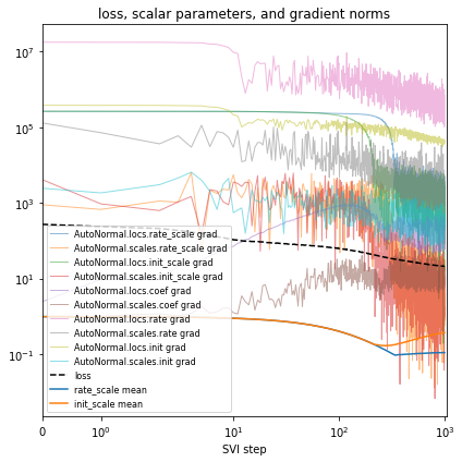
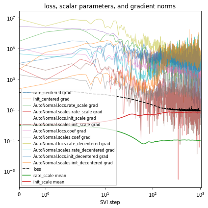
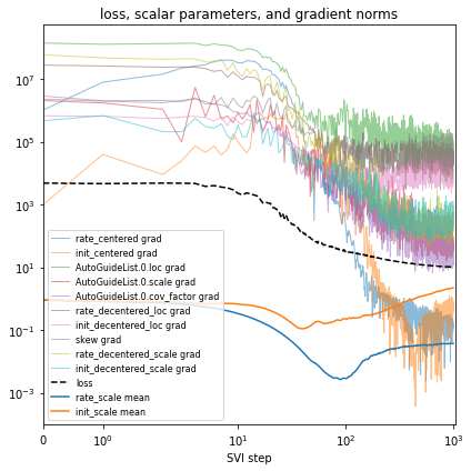
# Plot series to assess convergence.
if plot:
plt.figure(figsize=(6, 6))
for name, Y in series.items():
if name == "loss":
plt.plot(Y, "k--", label=name, zorder=0)
elif name.endswith(" mean"):
plt.plot(Y, label=name, zorder=-1)
else:
plt.plot(Y, label=name, alpha=0.5, lw=1, zorder=-2)
plt.xlabel("SVI step")
plt.title("loss, scalar parameters, and gradient norms")
plt.yscale("log")
plt.xscale("symlog")
plt.xlim(0, None)
plt.legend(loc="best", fontsize=8)
plt.tight_layout()
[7]:
%%time
guide = AutoNormal(model, init_scale=0.01)
fit_svi(model, guide)
Found 538452 latent variables and 1068600 learnable parameters
step    0 loss = 273.123
step  100 loss = 63.2423
step  200 loss = 44.9539
step  300 loss = 34.8813
step  400 loss = 30.4243
step  500 loss = 27.5258
step  600 loss = 25.4543
step  700 loss = 23.9134
step  800 loss = 22.7201
step  900 loss = 21.8574
step 1000 loss = 21.2031
CPU times: user 3min 4s, sys: 2min 48s, total: 5min 52s
Wall time: 1min 47s
After each change to the model or inference, you’ll validate model outputs, closing Box’s loop. In our running example we’ll quantitiatively evaluate using the mean average error (MAE) over the last fully-observed time step.
[8]:
def mae(true_counts, pred_probs):
    """Computes mean average error between counts and predicted probabilities."""
    pred_counts = pred_probs * true_counts.sum(-1, True)
    error = (true_counts - pred_counts).abs().sum(-1)
    total = true_counts.sum(-1).clamp(min=1)
    return (error / total).mean().item()

def evaluate(
    model, guide, num_particles=100, location="USA / Massachusetts", time=-2
):
    if smoke_test:
        num_particles = 4
    """Evaluate posterior predictive accuracy at the last fully observed time step."""
    with torch.no_grad(), poutine.mask(mask=False):  # makes computations cheaper
        with pyro.plate("particle", num_particles, dim=-3):  # vectorizes
            guide_trace = poutine.trace(guide).get_trace(dataset)
            probs = poutine.replay(model, guide_trace)(dataset, predict=time)
        probs = probs.squeeze().mean(0)  # average over Monte Carlo samples
        true_counts = dataset["counts"][time]
        # Compute global and local KL divergence.
        global_mae = mae(true_counts, probs)
        i = dataset["locations"].index(location)
        local_mae = mae(true_counts[i], probs[i])
    return {"MAE (global)": global_mae, f"MAE ({location})": local_mae}
[9]:
pprint(evaluate(model, guide))
{'MAE (USA / Massachusetts)': 0.26023179292678833,
 'MAE (global)': 0.22586050629615784}
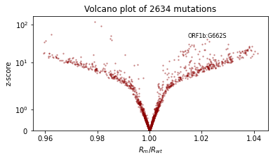
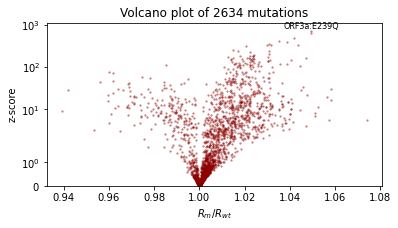
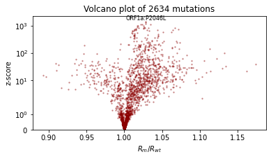
We’ll also qualitatively evaluate using a volcano plot showing the effect size and statistical significance of each mutation’s coefficient, and labeling the mutation with the most significant positive effect. We expect: - most mutations have very little effect (they are near zero in log space, so their multiplicative effect is near 1x) - more mutations have positive effect than netagive effect - effect sizes are on the order of 1.1 or 0.9.
[10]:
def plot_volcano(guide, num_particles=100):
    if smoke_test:
        num_particles = 4
    with torch.no_grad(), poutine.mask(mask=False):  # makes computations cheaper
        with pyro.plate("particle", num_particles, dim=-3):  # vectorizes
            trace = poutine.trace(guide).get_trace(dataset)
            trace = poutine.trace(poutine.replay(model, trace)).get_trace(dataset, -1)
            coef = trace.nodes["coef"]["value"].cpu()
    coef = coef.squeeze() * 0.01  # Scale factor as in the model.
    mean = coef.mean(0)
    std = coef.std(0)
    z_score = mean.abs() / std
    effect_size = mean.exp().numpy()
    plt.figure(figsize=(6, 3))
    plt.scatter(effect_size, z_score.numpy(), lw=0, s=5, alpha=0.5, color="darkred")
    plt.yscale("symlog")
    plt.ylim(0, None)
    plt.xlabel("$R_m/R_{wt}$")
    plt.ylabel("z-score")
    i = int((mean / std).max(0).indices)
    plt.text(effect_size[i], z_score[i] * 1.1, dataset["mutations"][i], ha="center", fontsize=8)
    plt.title(f"Volcano plot of {len(mean)} mutations")

plot_volcano(guide)
Create an initialization heuristic
In high-dimensional models, convergence can be slow and NANs arise easily, even when sampling from weakly informative priors. We recommend heuristically initializing a point estimate for each latent variable, aiming to initialize at something that is the right order of magnitude. Often you can initialize to a simple statistic of the data, e.g. a mean or standard deviation.
Pyro’s autoguides provide a number of `initialization strategies <>`__ for initializing the location parameter of many variational families, specified as init_loc_fn. You can create a custom initializer by accepting a pyro sample site dict and generating a sample from site["name"] and site["fn"] using e.g. site["fn"].shape(), site["fn"].support, site["fn"].mean, or sampling via site["fn"].sample().
[11]:
def init_loc_fn(site):
    shape = site["fn"].shape()
    if site["name"] == "coef":
        return torch.randn(shape).sub_(0.5).mul(0.01)
    if site["name"] == "init":
        # Heuristically initialize based on data.
        return dataset["counts"].mean(0).add(0.01).log()
    return init_to_feasible(site)  # fallback
As you evolve a model, you’ll add and remove and rename latent variables. We find it useful to require inits for all latent variables, add a message to remind yourself to udpate the init_loc_fn whenever the model changes.
[12]:
def init_loc_fn(site):
    shape = site["fn"].shape()
    if site["name"].endswith("_scale"):
        return torch.ones(shape)
    if site["name"] == "coef":
        return torch.randn(shape).sub_(0.5).mul(0.01)
    if site["name"] == "rate":
        return torch.zeros(shape)
    if site["name"] == "init":
        return dataset["counts"].mean(0).add(0.01).log()
    raise NotImplementedError(f"TODO initialize latent variable {site['name']}")
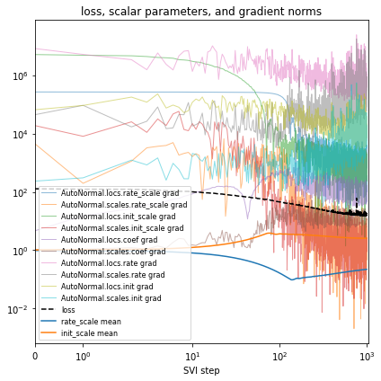
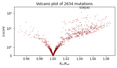
[13]:
%%time
guide = AutoNormal(model, init_loc_fn=init_loc_fn, init_scale=0.01)
fit_svi(model, guide, lr=0.02)
pprint(evaluate(model, guide))
plot_volcano(guide)
Found 538452 latent variables and 1068600 learnable parameters
step    0 loss = 127.475
step  100 loss = 44.9544
step  200 loss = 31.4236
step  300 loss = 24.4205
step  400 loss = 20.6802
step  500 loss = 18.6063
step  600 loss = 17.2365
step  700 loss = 16.5067
step  800 loss = 16.001
step  900 loss = 15.5123
step 1000 loss = 18.8275
{'MAE (USA / Massachusetts)': 0.29367634654045105,
 'MAE (global)': 0.2283070981502533}
CPU times: user 3min 17s, sys: 2min 51s, total: 6min 9s
Wall time: 1min 58s
Reparametrize the model
Reparametrizing a model preserves its distribution while changing its geometry. Reparametrizing is simply a change of coordinates. When reparametrizing we aim to warp a model’s geometry to remove correlations and to lift inconvenient topological manifolds into simpler higher dimensional flat Euclidean space.
Whereas many probabilistic programming languages require users to rewrite models to change coordinates, Pyro implements a library of about 15 different reparametrization effects including decentering (Gorinova et al. 2020), Haar wavelet transforms, and neural transport (Hoffman et al. 2019), as well as strategies to automatically apply effects and machinery to create custom reparametrization effects. Using these reparametrizers you can separate modeling from inference: first specify a model in a form that is natural to domain experts, then in inference code, reparametrize the model to have geometry that is more amenable to variational inference.
In our SARS-CoV-2 model, the geometry might improve if we change
- rate = pyro.sample("rate", dist.Normal(rate_loc, rate_scale))
+ rate = pyro.sample("rate", dist.Normal(0, 1)) * rate_scale + rate_loc
but that would make the model less interpretable. Instead we can reparametrize the model
[14]:
reparam_model = poutine.reparam(model, config={"rate": LocScaleReparam()})
or even automatically apply a set of recommended reparameterizers
[15]:
reparam_model = AutoReparam()(model)
Let’s try reparametrizing both sites “rate” and “init”. Note we’ll create a fresh reparam_model each time we train a guide, since the parameters are stored in that reparam_model instance. Take care to use the reparam_model in downstream prediction tasks like running evaluate(reparam_model, guide).
[16]:
%%time
reparam_model = poutine.reparam(
    model, {"rate": LocScaleReparam(), "init": LocScaleReparam()}
)
guide = AutoNormal(reparam_model, init_loc_fn=init_loc_fn, init_scale=0.01)
fit_svi(reparam_model, guide, lr=0.05)
pprint(evaluate(reparam_model, guide))
plot_volcano(guide)
Found 538452 latent variables and 1068602 learnable parameters
step    0 loss = 127.368
step  100 loss = 20.2831
step  200 loss = 11.0703
step  300 loss = 9.64594
step  400 loss = 9.52988
step  500 loss = 9.09012
step  600 loss = 9.25454
step  700 loss = 8.60661
step  800 loss = 8.9332
step  900 loss = 8.64206
step 1000 loss = 8.56663
{'MAE (USA / Massachusetts)': 0.1336274892091751,
 'MAE (global)': 0.1719919890165329}
CPU times: user 4min 21s, sys: 3min 9s, total: 7min 31s
Wall time: 2min 17s
Customize the variational family
When creating a new model, we recommend starting with mean field variational inference using an `AutoNormal <>`__ guide. This mean field guide is good at finding the neighborhood of your model’s mode, but naively it ignores correlations between latent variables. A first step in capturing correlations is to reparametrize the model as above: using a LocScaleReparam or HaarReparam (where appropriate) already allows the guide to capture some correlations among latent variables.
The next step towards modeling uncertainty is to customize the variational family by trying other autoguides, building on `EasyGuide <>`__, or creating a custom guide using Pyro primitives. We recommend increasing guide complexity gradually via these steps: 1. Start with an `AutoNormal <>`__ guide. 2. Try `AutoLowRankMultivariateNormal <>`__, which can model the principle components of correlated uncertainty. (For models with only ~100 latent variables you might also try
`AutoMultivariateNormal <>`__ or `AutoGaussian <>`__). 3. Try combining multiple guides using `AutoGuideList <>`__. For example if `AutoLowRankMultivariateNormal <>`__ is too expensive for all the latent variables, you can use `AutoGuideList <>`__ to combine an `AutoLowRankMultivariateNormal <>`__ guide over a few top-level global latent variables, together with a cheaper `AutoNormal <>`__ guide over more numerous local latent variables. 4. Try using `AutoGuideList <>`__ to combine a autoguide
together with a custom guide function built using pyro.sample, pyro.param, and pyro.plate. Given a partial_guide() function that covers just a few latent variables, you can AutoGuideList.append(partial_guide) just as you append autoguides. 5. Consider customizing one of Pyro’s autoguides that leverage model structure, e.g. AutoStructured,
AutoNormalMessenger, AutoHierarchicalNormalMessenger AutoRegressiveMessenger. 6. For models with local correlations, consider building on EasyGuide, a framework for building guides over
groups of variables.
While a fully-custom guides built from pyro.sample primitives offer the most flexible variational family, they are also the most brittle guides because each code change to the model or reparametrizer requires changes in the guide. The author recommends avoiding completely low-level guides and instead using AutoGuide or EasyGuide for at least some parts of the model, thereby speeding up model iteration.
Let’s first try a simple AutoLowRankMultivariateNormal guide.
[17]:
%%time
reparam_model = poutine.reparam(
    model, {"rate": LocScaleReparam(), "init": LocScaleReparam()}
)
guide = AutoLowRankMultivariateNormal(
    reparam_model, init_loc_fn=init_loc_fn, init_scale=0.01, rank=100
)
fit_svi(reparam_model, guide, num_steps=10, log_every=1, plot=False)
# don't even bother to evaluate, since this is too slow.
Found 538452 latent variables and 54498602 learnable parameters
step    0 loss = 128.329
step    1 loss = 126.172
step    2 loss = 124.691
step    3 loss = 123.609
step    4 loss = 123.317
step    5 loss = 121.567
step    6 loss = 120.513
step    7 loss = 121.759
step    8 loss = 120.844
step    9 loss = 121.641
CPU times: user 45.9 s, sys: 38.2 s, total: 1min 24s
Wall time: 29 s
Yikes! This is quite slow and sometimes runs out of memory on GPU.
Let’s make this cheaper by using AutoGuideList to combine an AutoLowRankMultivariateNormal guide over the most important variables rate_scale, init_scale, and coef, together with a simple cheap AutoNormal guide on the rest of the model (the expensive rate and init variables). The typical pattern is to create two views of the model with poutine.block, one exposing the target variables and
the other hiding them.
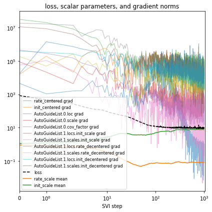
[18]:
%%time
reparam_model = poutine.reparam(
model, {"rate": LocScaleReparam(), "init": LocScaleReparam()}
)
guide = AutoGuideList(reparam_model)
mvn_vars = ["coef", "rate_scale", "coef_scale"]
guide.add(
AutoLowRankMultivariateNormal(
poutine.block(reparam_model, expose=mvn_vars),
init_loc_fn=init_loc_fn,
init_scale=0.01,
)
)
guide.add(
AutoNormal(
poutine.block(reparam_model, hide=mvn_vars),
init_loc_fn=init_loc_fn,
init_scale=0.01,
)
)
fit_svi(reparam_model, guide, lr=0.1)
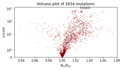
pprint(evaluate(reparam_model, guide))
plot_volcano(guide)
Found 538452 latent variables and 1202987 learnable parameters
step    0 loss = 832.956
step  100 loss = 11.9687
step  200 loss = 11.1152
step  300 loss = 9.60629
step  400 loss = 10.1724
step  500 loss = 9.18063
step  600 loss = 9.1669
step  700 loss = 9.06247
step  800 loss = 9.38853
step  900 loss = 9.12489
step 1000 loss = 8.93582
{'MAE (USA / Massachusetts)': 0.09685955196619034,
 'MAE (global)': 0.16698431968688965}
CPU times: user 4min 22s, sys: 3min 5s, total: 7min 28s
Wall time: 2min 15s
Next let’s create a custom guide for part of the model, just the rate and init parts. Since we’ll want to use this with reparametrizers, we’ll make the guide use the auxiliary latent variables created by poutine.reparam, rather than the original rate and init variables. Let’s see what these variables are named:
[19]:
for name, site in poutine.trace(reparam_model).get_trace(
    dataset
).iter_stochastic_nodes():
    print(name)
rate_scale
init_scale
mutation
coef
strain
place
rate_decentered
init_decentered
It looks like these new auxiliary variables are called rate_decentered and init_decentered.
[20]:
def local_guide(dataset):
    # Create learnable parameters.
    T, P, S = dataset["counts"].shape
    r_loc = pyro.param("rate_decentered_loc", lambda: torch.zeros(P, S))
    i_loc = pyro.param("init_decentered_loc", lambda: torch.zeros(P, S))
    skew = pyro.param("skew", lambda: torch.zeros(P, S))  # allows correlation
    r_scale = pyro.param("rate_decentered_scale", lambda: torch.ones(P, S),
                          constraint=constraints.softplus_positive)
    i_scale = pyro.param("init_decentered_scale", lambda: torch.ones(P, S),
                          constraint=constraints.softplus_positive)

    # Sample local variables inside plates.
    # Note plates are already created by the main guide, so we'll
    # use the existing plates rather than calling pyro.plate(...).
    with guide.plates["place"], guide.plates["strain"]:
        samples = {}
        samples["rate_decentered"] = pyro.sample(
            "rate_decentered", dist.Normal(r_loc, r_scale)
        )
        i_loc = i_loc + skew * samples["rate_decentered"]
        samples["init_decentered"] = pyro.sample(
            "init_decentered", dist.Normal(i_loc, i_scale)
        )
    return samples
[21]:
%%time
reparam_model = poutine.reparam(
    model, {"rate": LocScaleReparam(), "init": LocScaleReparam()}
)
guide = AutoGuideList(reparam_model)
local_vars = ["rate_decentered", "init_decentered"]
guide.add(
    AutoLowRankMultivariateNormal(
        poutine.block(reparam_model, hide=local_vars),
        init_loc_fn=init_loc_fn,
        init_scale=0.01,
    )
)
guide.add(local_guide)
fit_svi(reparam_model, guide, lr=0.1)
pprint(evaluate(reparam_model, guide))
plot_volcano(guide)
Found 538452 latent variables and 1468870 learnable parameters
step    0 loss = 4804.42
step  100 loss = 31.7409
step  200 loss = 19.8206
step  300 loss = 15.2961
step  400 loss = 13.2222
step  500 loss = 12.1435
step  600 loss = 11.4291
step  700 loss = 10.9722
step  800 loss = 10.6209
step  900 loss = 10.3649
step 1000 loss = 10.1804
{'MAE (USA / Massachusetts)': 0.1159871369600296,
 'MAE (global)': 0.1876191794872284}
CPU times: user 4min 26s, sys: 3min 7s, total: 7min 33s
Wall time: 2min 18s
Conclusion
We’ve seen how to use initialization, reparameterization, autoguides, and custom guides in a Bayesian workflow. For more examples of these pieces of machinery, we recommend exploring the Pyro codebase, e.g. search for “poutine.reparam” or “init_loc_fn” in the Pyro codebase.
[ ]: