Forecasting II: state space models
This tutorial covers state space modeling with the pyro.contrib.forecast module. This tutorial assumes the reader is already familiar with SVI, tensor shapes, and univariate forecasting.
See also:
Summary
Pyro’s ForecastingModel can combine regression, variational inference, and exact inference.
To model a linear-Gaussian dynamical system, use a GaussianHMM
noise_dist.To model a heavy-tailed linear dynamical system, use LinearHMM with heavy-tailed distributions.
To enable inference with LinearHMM, use a LinearHMMReparam reparameterizer.
[1]:
import math
import torch
import pyro
import pyro.distributions as dist
import pyro.poutine as poutine
from pyro.contrib.examples.bart import load_bart_od
from pyro.contrib.forecast import ForecastingModel, Forecaster, eval_crps
from pyro.infer.reparam import LinearHMMReparam, StableReparam, SymmetricStableReparam
from pyro.ops.tensor_utils import periodic_repeat
from pyro.ops.stats import quantile
import matplotlib.pyplot as plt

%matplotlib inline
assert pyro.__version__.startswith('1.9.1')
pyro.set_rng_seed(20200305)
Intro to state space models
In the univariate tutorial we saw how to model time series as regression plus a local level model, using variational inference. This tutorial covers a different way to model time series: state space models and exact inference. Pyro’s forecasting module allows these two paradigms to be combined, for example modeling seasonality with regression, including a slow global trend, and using a state-space model for short-term local trend.
Pyro implements a few state space models, but the most important are the GaussianHMM distribution and its heavy-tailed generalization the LinearHMM distribution. Both of these model a linear dynamical system with hidden state; both are multivariate, and both allow learning of all process parameters. On top of these the
pyro.contrib.timeseries module implements a variety of multivariate Gaussian Process models that compile down to GaussianHMMs.
Pyro’s inference for GaussianHMM uses parallel-scan Kalman filtering, allowing fast analysis of very long time series. Similarly, Pyro’s inference for LinearHMM uses entirely parallel auxiliary variable methods to reduce to a GaussianHMM, which then permits parallel-scan inference. Thus both methods allow parallelization of long time series analysis, even for a single univariate time series.
Let’s again look at the BART train ridership dataset:
[2]:
dataset = load_bart_od()
print(dataset.keys())
print(dataset["counts"].shape)
print(" ".join(dataset["stations"]))
dict_keys(['stations', 'start_date', 'counts'])
torch.Size([78888, 50, 50])
12TH 16TH 19TH 24TH ANTC ASHB BALB BAYF BERY CAST CIVC COLM COLS CONC DALY DBRK DELN DUBL EMBR FRMT FTVL GLEN HAYW LAFY LAKE MCAR MLBR MLPT MONT NBRK NCON OAKL ORIN PCTR PHIL PITT PLZA POWL RICH ROCK SANL SBRN SFIA SHAY SSAN UCTY WARM WCRK WDUB WOAK
[3]:
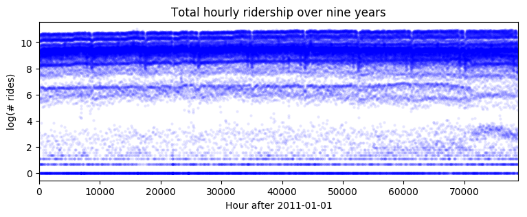
data = dataset["counts"].sum([-1, -2]).unsqueeze(-1).log1p()
print(data.shape)
plt.figure(figsize=(9, 3))
plt.plot(data, 'b.', alpha=0.1, markeredgewidth=0)
plt.title("Total hourly ridership over nine years")
plt.ylabel("log(# rides)")
plt.xlabel("Hour after 2011-01-01")
plt.xlim(0, len(data));
torch.Size([78888, 1])
[4]:
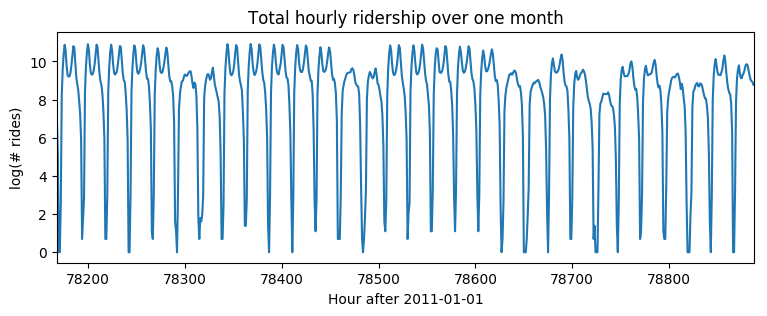
plt.figure(figsize=(9, 3))
plt.plot(data)
plt.title("Total hourly ridership over one month")
plt.ylabel("log(# rides)")
plt.xlabel("Hour after 2011-01-01")
plt.xlim(len(data) - 24 * 30, len(data));
GaussianHMM
Let’s start by modeling hourly seasonality together with a local linear trend, where we model seasonality via regression and local linear trend via a GaussianHMM. This noise model includes a mean-reverting hidden state (an Ornstein-Uhlenbeck process) plus Gaussian observation noise.
[5]:
T0 = 0                # beginning
T2 = data.size(-2)    # end
T1 = T2 - 24 * 7 * 2  # train/test split
means = data[:T1 // (24 * 7) * 24 * 7].reshape(-1, 24 * 7).mean(0)
[6]:
class Model1(ForecastingModel):
    def model(self, zero_data, covariates):
        duration = zero_data.size(-2)

        # We'll hard-code the periodic part of this model, learning only the local model.
        prediction = periodic_repeat(means, duration, dim=-1).unsqueeze(-1)

        # On top of this mean prediction, we'll learn a linear dynamical system.
        # This requires specifying five pieces of data, on which we will put structured priors.
        init_dist = dist.Normal(0, 10).expand([1]).to_event(1)

        timescale = pyro.sample("timescale", dist.LogNormal(math.log(24), 1))
        # Note timescale is a scalar but we need a 1x1 transition matrix (hidden_dim=1),
        # thus we unsqueeze twice using [..., None, None].
        trans_matrix = torch.exp(-1 / timescale)[..., None, None]
        trans_scale = pyro.sample("trans_scale", dist.LogNormal(-0.5 * math.log(24), 1))
        trans_dist = dist.Normal(0, trans_scale.unsqueeze(-1)).to_event(1)

        # Note the obs_matrix has shape hidden_dim x obs_dim = 1 x 1.
        obs_matrix = torch.tensor([[1.]])
        obs_scale = pyro.sample("obs_scale", dist.LogNormal(-2, 1))
        obs_dist = dist.Normal(0, obs_scale.unsqueeze(-1)).to_event(1)

        noise_dist = dist.GaussianHMM(
            init_dist, trans_matrix, trans_dist, obs_matrix, obs_dist, duration=duration)
        self.predict(noise_dist, prediction)
We can then train the model on many years of data. Note that because we are being variational about only time-global variables, and exactly integrating out time-local variables (via GaussianHMM), stochastic gradients are very low variance; this allows us to use a large learning rate and few steps.
[7]:
%%time
pyro.set_rng_seed(1)
pyro.clear_param_store()
covariates = torch.zeros(len(data), 0)  # empty
forecaster = Forecaster(Model1(), data[:T1], covariates[:T1], learning_rate=0.1, num_steps=400)
for name, value in forecaster.guide.median().items():
    if value.numel() == 1:
        print("{} = {:0.4g}".format(name, value.item()))
INFO     step    0 loss = 0.878717
INFO     step  100 loss = 0.650493
INFO     step  200 loss = 0.650542
INFO     step  300 loss = 0.650579
timescale = 4.461
trans_scale = 0.4563
obs_scale = 0.0593
CPU times: user 26.3 s, sys: 1.47 s, total: 27.8 s
Wall time: 27.8 s
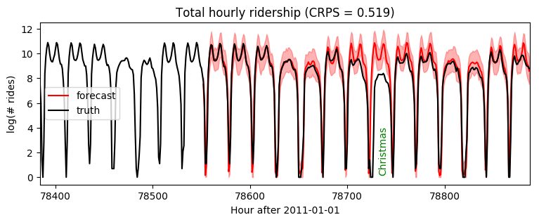
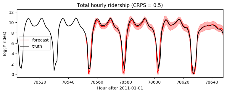
Plotting forecasts of the next two weeks of data, we see mostly reasonable forecasts, but an anomaly on Christmas when rides were overpredicted. This is to be expected, as we have not modeled yearly seasonality or holidays.
[8]:
samples = forecaster(data[:T1], covariates, num_samples=100)
samples.clamp_(min=0)  # apply domain knowledge: the samples must be positive
p10, p50, p90 = quantile(samples, (0.1, 0.5, 0.9)).squeeze(-1)
crps = eval_crps(samples, data[T1:])
print(samples.shape, p10.shape)

plt.figure(figsize=(9, 3))
plt.fill_between(torch.arange(T1, T2), p10, p90, color="red", alpha=0.3)
plt.plot(torch.arange(T1, T2), p50, 'r-', label='forecast')
plt.plot(torch.arange(T1 - 24 * 7, T2),
         data[T1 - 24 * 7: T2], 'k-', label='truth')
plt.title("Total hourly ridership (CRPS = {:0.3g})".format(crps))
plt.ylabel("log(# rides)")
plt.xlabel("Hour after 2011-01-01")
plt.xlim(T1 - 24 * 7, T2)
plt.text(78732, 3.5, "Christmas", rotation=90, color="green")
plt.legend(loc="best");
torch.Size([100, 336, 1]) torch.Size([336])
Next let’s change the model to use heteroskedastic observation noise, depending on the hour of week.
[9]:
class Model2(ForecastingModel):
    def model(self, zero_data, covariates):
        duration = zero_data.size(-2)
        prediction = periodic_repeat(means, duration, dim=-1).unsqueeze(-1)

        init_dist = dist.Normal(0, 10).expand([1]).to_event(1)
        timescale = pyro.sample("timescale", dist.LogNormal(math.log(24), 1))
        trans_matrix = torch.exp(-1 / timescale)[..., None, None]
        trans_scale = pyro.sample("trans_scale", dist.LogNormal(-0.5 * math.log(24), 1))
        trans_dist = dist.Normal(0, trans_scale.unsqueeze(-1)).to_event(1)
        obs_matrix = torch.tensor([[1.]])

        # To model heteroskedastic observation noise, we'll sample obs_scale inside a plate,
        # then repeat to full duration. This is the only change from Model1.
        with pyro.plate("hour_of_week", 24 * 7, dim=-1):
            obs_scale = pyro.sample("obs_scale", dist.LogNormal(-2, 1))
        obs_scale = periodic_repeat(obs_scale, duration, dim=-1)

        obs_dist = dist.Normal(0, obs_scale.unsqueeze(-1)).to_event(1)
        noise_dist = dist.GaussianHMM(
            init_dist, trans_matrix, trans_dist, obs_matrix, obs_dist, duration=duration)
        self.predict(noise_dist, prediction)
[10]:
%%time
pyro.set_rng_seed(1)
pyro.clear_param_store()
covariates = torch.zeros(len(data), 0)  # empty
forecaster = Forecaster(Model2(), data[:T1], covariates[:T1], learning_rate=0.1, num_steps=400)
for name, value in forecaster.guide.median().items():
    if value.numel() == 1:
        print("{} = {:0.4g}".format(name, value.item()))
INFO     step    0 loss = 0.954783
INFO     step  100 loss = -0.0344435
INFO     step  200 loss = -0.0373581
INFO     step  300 loss = -0.0376129
timescale = 61.41
trans_scale = 0.1082
CPU times: user 28.1 s, sys: 1.34 s, total: 29.5 s
Wall time: 29.6 s
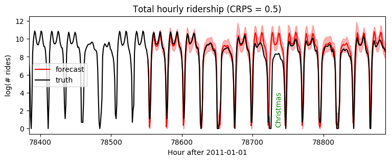
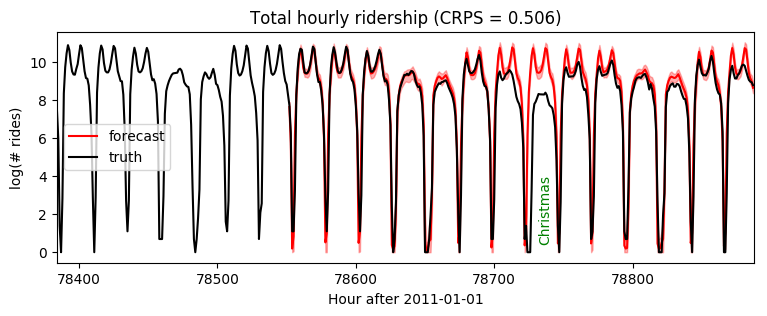
Note this gives us a much longer timescale and thereby more accurate short-term predictions:
[11]:
samples = forecaster(data[:T1], covariates, num_samples=100)
samples.clamp_(min=0)  # apply domain knowledge: the samples must be positive
p10, p50, p90 = quantile(samples, (0.1, 0.5, 0.9)).squeeze(-1)
crps = eval_crps(samples, data[T1:])

plt.figure(figsize=(9, 3))
plt.fill_between(torch.arange(T1, T2), p10, p90, color="red", alpha=0.3)
plt.plot(torch.arange(T1, T2), p50, 'r-', label='forecast')
plt.plot(torch.arange(T1 - 24 * 7, T2),
         data[T1 - 24 * 7: T2], 'k-', label='truth')
plt.title("Total hourly ridership (CRPS = {:0.3g})".format(crps))
plt.ylabel("log(# rides)")
plt.xlabel("Hour after 2011-01-01")
plt.xlim(T1 - 24 * 7, T2)
plt.text(78732, 3.5, "Christmas", rotation=90, color="green")
plt.legend(loc="best");
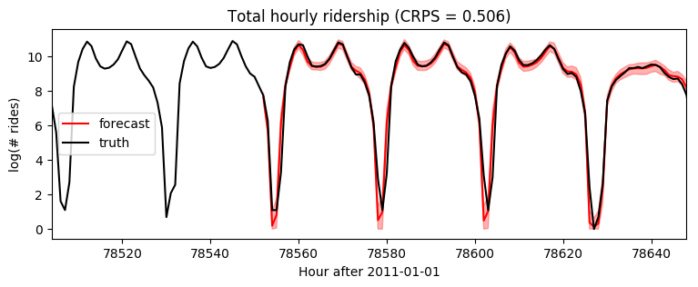
[12]:
plt.figure(figsize=(9, 3))
plt.fill_between(torch.arange(T1, T2), p10, p90, color="red", alpha=0.3)
plt.plot(torch.arange(T1, T2), p50, 'r-', label='forecast')
plt.plot(torch.arange(T1 - 24 * 7, T2),
         data[T1 - 24 * 7: T2], 'k-', label='truth')
plt.title("Total hourly ridership (CRPS = {:0.3g})".format(crps))
plt.ylabel("log(# rides)")
plt.xlabel("Hour after 2011-01-01")
plt.xlim(T1 - 24 * 2, T1 + 24 * 4)
plt.legend(loc="best");
Heavy-tailed modeling with LinearHMM
Next let’s change our model to a linear-Stable dynamical system, exhibiting learnable heavy tailed behavior in both the process noise and observation noise. As we’ve already seen in the univariate tutorial, this will require special handling of stable distributions by poutine.reparam(). For state space models, we combine LinearHMMReparam with other reparameterizers like StableReparam and SymmetricStableReparam. All reparameterizers preserve behavior of the generative model, and only serve to enable inference via auxiliary variable methods.
[13]:
class Model3(ForecastingModel):
    def model(self, zero_data, covariates):
        duration = zero_data.size(-2)
        prediction = periodic_repeat(means, duration, dim=-1).unsqueeze(-1)

        # First sample the Gaussian-like parameters as in previous models.
        init_dist = dist.Normal(0, 10).expand([1]).to_event(1)
        timescale = pyro.sample("timescale", dist.LogNormal(math.log(24), 1))
        trans_matrix = torch.exp(-1 / timescale)[..., None, None]
        trans_scale = pyro.sample("trans_scale", dist.LogNormal(-0.5 * math.log(24), 1))
        obs_matrix = torch.tensor([[1.]])
        with pyro.plate("hour_of_week", 24 * 7, dim=-1):
            obs_scale = pyro.sample("obs_scale", dist.LogNormal(-2, 1))
        obs_scale = periodic_repeat(obs_scale, duration, dim=-1)

        # In addition to the Gaussian parameters, we will learn a global stability
        # parameter to determine tail weights, and an observation skew parameter.
        stability = pyro.sample("stability", dist.Uniform(1, 2).expand([1]).to_event(1))
        skew = pyro.sample("skew", dist.Uniform(-1, 1).expand([1]).to_event(1))

        # Next we construct stable distributions and a linear-stable HMM distribution.
        trans_dist = dist.Stable(stability, 0, trans_scale.unsqueeze(-1)).to_event(1)
        obs_dist = dist.Stable(stability, skew, obs_scale.unsqueeze(-1)).to_event(1)
        noise_dist = dist.LinearHMM(
            init_dist, trans_matrix, trans_dist, obs_matrix, obs_dist, duration=duration)

        # Finally we use a reparameterizer to enable inference.
        rep = LinearHMMReparam(None,                     # init_dist is already Gaussian.
                               SymmetricStableReparam(), # trans_dist is symmetric.
                               StableReparam())          # obs_dist is asymmetric.
        with poutine.reparam(config={"residual": rep}):
            self.predict(noise_dist, prediction)
Note that since this model introduces auxiliary variables that are learned by variational inference, gradients are higher variance and we need to train for longer.
[14]:
%%time
pyro.set_rng_seed(1)
pyro.clear_param_store()
covariates = torch.zeros(len(data), 0)  # empty
forecaster = Forecaster(Model3(), data[:T1], covariates[:T1], learning_rate=0.1)
for name, value in forecaster.guide.median().items():
    if value.numel() == 1:
        print("{} = {:0.4g}".format(name, value.item()))
INFO     step    0 loss = 42.9188
INFO     step  100 loss = 0.243742
INFO     step  200 loss = 0.112491
INFO     step  300 loss = 0.0320302
INFO     step  400 loss = -0.0424252
INFO     step  500 loss = -0.0763611
INFO     step  600 loss = -0.108585
INFO     step  700 loss = -0.129246
INFO     step  800 loss = -0.143037
INFO     step  900 loss = -0.173499
INFO     step 1000 loss = -0.172329
timescale = 11.29
trans_scale = 0.04193
stability = 1.68
skew = -0.0001891
CPU times: user 2min 57s, sys: 21.9 s, total: 3min 19s
Wall time: 3min 19s
[15]:
samples = forecaster(data[:T1], covariates, num_samples=100)
samples.clamp_(min=0)  # apply domain knowledge: the samples must be positive
p10, p50, p90 = quantile(samples, (0.1, 0.5, 0.9)).squeeze(-1)
crps = eval_crps(samples, data[T1:])

plt.figure(figsize=(9, 3))
plt.fill_between(torch.arange(T1, T2), p10, p90, color="red", alpha=0.3)
plt.plot(torch.arange(T1, T2), p50, 'r-', label='forecast')
plt.plot(torch.arange(T1 - 24 * 7, T2),
         data[T1 - 24 * 7: T2], 'k-', label='truth')
plt.title("Total hourly ridership (CRPS = {:0.3g})".format(crps))
plt.ylabel("log(# rides)")
plt.xlabel("Hour after 2011-01-01")
plt.xlim(T1 - 24 * 7, T2)
plt.text(78732, 3.5, "Christmas", rotation=90, color="green")
plt.legend(loc="best");
[16]:
plt.figure(figsize=(9, 3))
plt.fill_between(torch.arange(T1, T2), p10, p90, color="red", alpha=0.3)
plt.plot(torch.arange(T1, T2), p50, 'r-', label='forecast')
plt.plot(torch.arange(T1 - 24 * 7, T2),
         data[T1 - 24 * 7: T2], 'k-', label='truth')
plt.title("Total hourly ridership (CRPS = {:0.3g})".format(crps))
plt.ylabel("log(# rides)")
plt.xlabel("Hour after 2011-01-01")
plt.xlim(T1 - 24 * 2, T1 + 24 * 4)
plt.legend(loc="best");
[ ]: