The Semi-Supervised VAE

Introduction

Most of the models we’ve covered in the tutorials are unsupervised:

• Variational Autoencoder (VAE)

• DMM

• Attend-Infer-Repeat

We’ve also covered a simple supervised model:

• Bayesian Regression

The semi-supervised setting represents an interesting intermediate case where some of the data is labeled and some is not. It is also of great practical importance, since we often have very little labeled data and much more unlabeled data. We’d clearly like to leverage labeled data to improve our models of the unlabeled data.

The semi-supervised setting is also well suited to generative models, where missing data can be accounted for quite naturally—at least conceptually. As we will see, in restricting our attention to semi-supervised generative models, there will be no shortage of different model variants and possible inference strategies. Although we’ll only be able to explore a few of these variants in detail, hopefully you will come away from the tutorial with a greater appreciation for the abstractions and modularity offered by probabilistic programming.

So let’s go about building a generative model. We have a dataset $\mathcal{D}$ with $N$ datapoints,

$$\mathcal{D}=\{({\mathbf{x}}_i,{\mathbf{y}}_i)\}$$

where the $\{{\mathbf{x}}_i\}$ are always observed and the labels $\{{\mathbf{y}}_i\}$ are only observed for some subset of the data. Since we want to be able to model complex variations in the data, we’re going to make this a latent variable model with a local latent variable ${\mathbf{z}}_i$ private to each pair $({\mathbf{x}}_i,{\mathbf{y}}_i)$. Even with this set of choices, a number of model variants are possible: we’re going to focus on the model variant depicted in Figure 1 (this is model M2 in reference [1]).

Figure 1: our semi-supervised generative model (c.f. model M2 in reference [1])

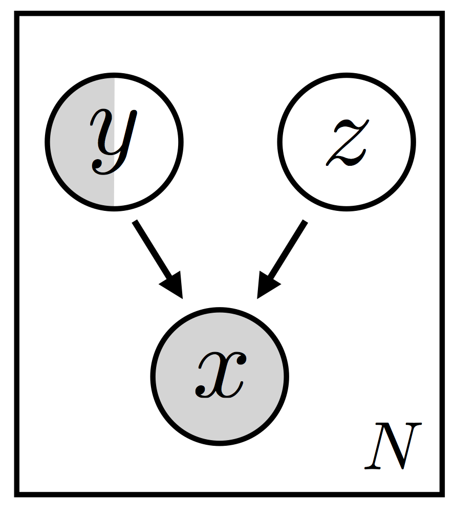
For convenience—and since we’re going to model MNIST in our experiments below—let’s suppose the $\{{\mathbf{x}}_i\}$ are images and the $\{{\mathbf{y}}_i\}$ are digit labels. In this model setup, the latent random variable ${\mathbf{z}}_i$ and the (partially observed) digit label jointly generate the observed image. The ${\mathbf{z}}_i$ represents everything but the digit label, possibly handwriting style or position. Let’s sidestep asking when we expect this particular factorization of $({\mathbf{x}}_i,{\mathbf{y}}_i,{\mathbf{z}}_i)$ to be appropriate, since the answer to that question will depend in large part on the dataset in question (among other things). Let’s instead highlight some of the ways that inference in this model will be challenging as well as some of the solutions that we’ll be exploring in the rest of the tutorial.

The Challenges of Inference

For concreteness we’re going to continue to assume that the partially-observed $\{{\mathbf{y}}_i\}$ are discrete labels; we will also assume that the $\{{\mathbf{z}}_i\}$ are continuous.

• If we apply the general recipe for stochastic variational inference to our model (see SVI Part I) we would be sampling the discrete (and thus non-reparameterizable) variable ${\mathbf{y}}_i$ whenever it’s unobserved. As discussed in SVI Part III this will generally lead to high-variance gradient estimates.

• A common way to ameliorate this problem—and one that we’ll explore below—is to forego sampling and instead sum out all ten values of the class label ${\mathbf{y}}_i$ when we calculate the ELBO for an unlabeled datapoint ${\mathbf{x}}_i$. This is more expensive per step, but can help us reduce the variance of our gradient estimator and thereby take fewer steps.

• Recall that the role of the guide is to ‘fill in’ latent random variables. Concretely, one component of our guide will be a digit classifier $q_{\varphi }(\mathbf{y}|\mathbf{x})$ that will randomly ‘fill in’ labels $\{{\mathbf{y}}_i\}$ given an image $\{{\mathbf{x}}_i\}$. Crucially, this means that the only term in the ELBO that will depend on $q_{\varphi }(\cdot |\mathbf{x})$ is the term that involves a sum over unlabeled datapoints. This means that our classifier $q_{\varphi }(\cdot |\mathbf{x})$—which in many cases will be the primary object of interest—will not be learning from the labeled datapoints (at least not directly).

• This seems like a potential problem. Luckily, various fixes are possible. Below we’ll follow the approach in reference [1], which involves introducing an additional objective function for the classifier to ensure that the classifier learns directly from the labeled data.

We have our work cut out for us so let’s get started!

First Variant: Standard objective function, naive estimator

As discussed in the introduction, we’re considering the model depicted in Figure 1. In more detail, the model has the following structure:

• $p(\mathbf{y})=Cat(\mathbf{y}|\pi )$: multinomial (or categorical) prior for the class label

• $p(\mathbf{z})=\mathcal{N}(\mathbf{z}|\mathbf{0}\mathbf{,}\mathbf{I})$: unit normal prior for the latent code $\mathbf{z}$

• $p_{\theta }(\mathbf{x}|\mathbf{z}\mathbf{,}\mathbf{y})=Bernoulli\left(\mathbf{x}|\mu \left(\mathbf{z}\mathbf{,}\mathbf{y}\right)\right)$: parameterized Bernoulli likelihood function; $\mu \left(\mathbf{z}\mathbf{,}\mathbf{y}\right)$ corresponds to decoder in the code

We structure the components of our guide $q_{\varphi }(.)$ as follows:

• $q_{\varphi }(\mathbf{y}|\mathbf{x})=Cat(\mathbf{y}|{\alpha }_{\varphi }\left(\mathbf{x}\right))$: parameterized multinomial (or categorical) distribution; ${\alpha }_{\varphi }\left(\mathbf{x}\right)$ corresponds to encoder_y in the code

• $q_{\varphi }(\mathbf{z}|\mathbf{x}\mathbf{,}\mathbf{y})=\mathcal{N}(\mathbf{z}|{\mu }_{\varphi }\left(\mathbf{x}\mathbf{,}\mathbf{y}\right),{\sigma }_{\varphi }^{\mathbf{2}}(\mathbf{x}\mathbf{,}\mathbf{y}))$: parameterized normal distribution; ${\mu }_{\varphi }\left(\mathbf{x}\mathbf{,}\mathbf{y}\right)$ and ${\sigma }_{\varphi }^{\mathbf{2}}(\mathbf{x}\mathbf{,}\mathbf{y})$ correspond to the neural digit classifier encoder_z in the code

These choices reproduce the structure of model M2 and its corresponding inference network in reference [1].

We translate this model and guide pair into Pyro code below. Note that:

• The labels ys, which are represented with a one-hot encoding, are only partially observed (None denotes unobserved values).

• model() handles both the observed and unobserved case.

• The code assumes that xs and ys are mini-batches of images and labels, respectively, with the size of each batch denoted by batch_size.

def model(self, xs, ys=None):
    # register this pytorch module and all of its sub-modules with pyro
    pyro.module("ss_vae", self)
    batch_size = xs.size(0)

    # inform Pyro that the variables in the batch of xs, ys are conditionally independent
    with pyro.plate("data"):

        # sample the handwriting style from the constant prior distribution
        prior_loc = xs.new_zeros([batch_size, self.z_dim])
        prior_scale = xs.new_ones([batch_size, self.z_dim])
        zs = pyro.sample("z", dist.Normal(prior_loc, prior_scale).to_event(1))

        # if the label y (which digit to write) is supervised, sample from the
        # constant prior, otherwise, observe the value (i.e. score it against the constant prior)
        alpha_prior = xs.new_ones([batch_size, self.output_size]) / (1.0 * self.output_size)
        ys = pyro.sample("y", dist.OneHotCategorical(alpha_prior), obs=ys)

        # finally, score the image (x) using the handwriting style (z) and
        # the class label y (which digit to write) against the
        # parametrized distribution p(x|y,z) = bernoulli(decoder(y,z))
        # where `decoder` is a neural network
        loc = self.decoder([zs, ys])
        pyro.sample("x", dist.Bernoulli(loc).to_event(1), obs=xs)

def guide(self, xs, ys=None):
    with pyro.plate("data"):
        # if the class label (the digit) is not supervised, sample
        # (and score) the digit with the variational distribution
        # q(y|x) = categorical(alpha(x))
        if ys is None:
            alpha = self.encoder_y(xs)
            ys = pyro.sample("y", dist.OneHotCategorical(alpha))

        # sample (and score) the latent handwriting-style with the variational
        # distribution q(z|x,y) = normal(loc(x,y),scale(x,y))
        loc, scale = self.encoder_z([xs, ys])
        pyro.sample("z", dist.Normal(loc, scale).to_event(1))

Network Definitions

In our experiments we use the same network configurations as used in reference [1]. The encoder and decoder networks have one hidden layer with $500$ hidden units and softplus activation functions. We use softmax as the activation function for the output of encoder_y, sigmoid as the output activation function for decoder and exponentiation for the scale part of the output of encoder_z. The latent dimension is 50.

MNIST Pre-Processing

We normalize the pixel values to the range $[0.0,1.0]$. We use the MNIST data loader from the torchvision library. The testing set consists of $10000$ examples. The default training set consists of $60000$ examples. We use the first $50000$ examples for training (divided into supervised and un-supervised parts) and the remaining $10000$ images for validation. For our experiments, we use $4$ configurations of supervision in the training set, i.e. we consider $3000$, $1000$, $600$ and $100$ supervised examples selected randomly (while ensuring that each class is balanced).

The Objective Function

The objective function for this model has the two terms (c.f. Eqn. 8 in reference [1]):

$$\mathcal{J}=\sum _{(\mathbf{x}\mathbf{,}\mathbf{y})\in {\mathcal{D}}_{supervised}}\mathcal{L}(\mathbf{x}\mathbf{,}\mathbf{y})+\sum _{\mathbf{x}\in {\mathcal{D}}_{unsupervised}}\mathcal{U}\left(\mathbf{x}\right)$$

To implement this in Pyro, we setup a single instance of the SVI class. The two different terms in the objective functions will emerge automatically depending on whether we pass the step method labeled or unlabeled data. We will alternate taking steps with labeled and unlabeled mini-batches, with the number of steps taken for each type of mini-batch depending on the total fraction of data that is labeled. For example, if we have 1,000 labeled images and 49,000 unlabeled ones, then we’ll take 49 steps with unlabeled mini-batches for each labeled mini-batch. (Note that there are different ways we could do this, but for simplicity we only consider this variant.) The code for this setup is given below:

from pyro.infer import SVI, Trace_ELBO, TraceEnum_ELBO, config_enumerate
from pyro.optim import Adam

# setup the optimizer
adam_params = {"lr": 0.0003}
optimizer = Adam(adam_params)

# setup the inference algorithm
svi = SVI(model, guide, optimizer, loss=Trace_ELBO())

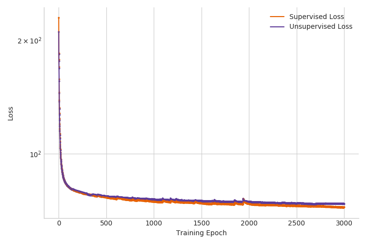
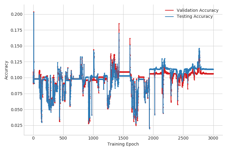
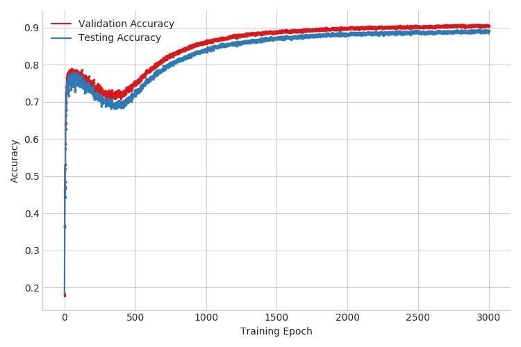
When we run this inference in Pyro, the performance seen during test time is degraded by the noise inherent in the sampling of the categorical variables (see Figure 2 and Table 1 at the end of this tutorial). To deal with this we’re going to need a better ELBO gradient estimator.

Figure 2: Variant 1 (Left) Training losses for the case with 3000 supervised examples. (Right) Test and validation accuracies.

Interlude: Summing Out Discrete Latents

As highlighted in the introduction, when the discrete latent labels $\mathbf{y}$ are not observed, the ELBO gradient estimates rely on sampling from $q_{\varphi }(\mathbf{y}|\mathbf{x})$. These gradient estimates can be very high-variance, especially early in the learning process when the guessed labels are often incorrect. A common approach to reduce variance in this case is to sum out discrete latent variables, replacing the Monte Carlo expectation

$${\mathbb{E}}_{\mathbf{y}\sim q_{\varphi }(\cdot |\mathbf{x})}\mathrm{\nabla }\mathrm{ELBO}$$

with an explicit sum

$$\sum _{\mathbf{y}}{q}_{\varphi }(\mathbf{y}|\mathbf{x})\mathrm{\nabla }\mathrm{ELBO}$$

This sum is usually implemented by hand, as in [1], but Pyro can automate this in many cases. To automatically sum out all discrete latent variables (here only $\mathbf{y}$), we simply wrap the guide in config_enumerate():

svi = SVI(model, config_enumerate(guide), optimizer, loss=TraceEnum_ELBO(max_plate_nesting=1))

In this mode of operation, each svi.step(...) computes a gradient term for each of the ten latent states of $y$. Although each step is thus $10\times$ more expensive, we’ll see that the lower-variance gradient estimate outweighs the additional cost.

Going beyond the particular model in this tutorial, Pyro supports summing over arbitrarily many discrete latent variables. Beware that the cost of summing is exponential in the number of discrete variables, but is cheap(er) if multiple independent discrete variables are packed into a single tensor (as in this tutorial, where the discrete labels for the entire mini-batch are packed into the single tensor $\mathbf{y}$). To use this parallel form of config_enumerate(), we must inform Pyro that the items in a minibatch are indeed independent by wrapping our vectorized code in a with pyro.plate("name") block.

Second Variant: Standard Objective Function, Better Estimator

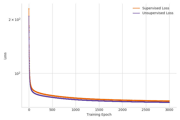
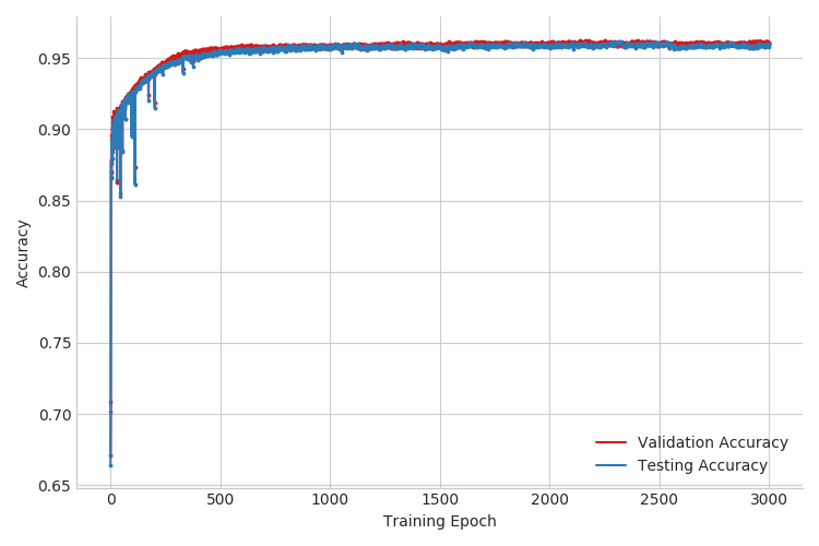
Now that we have the tools to sum out discrete latents, we can see if doing so helps our performance. First, as we can see from Figure 3, the test and validation accuracies now evolve much more smoothly over the course of training. More importantly, this single modification improved test accuracy from around 20% to about 90% for the case of $3000$ labeled examples. See Table 1 for the full results. This is great, but can we do better?

Figure 3: Variant 2 (Left) Training losses for the case with 3000 supervised examples. (Right) Test and validation accuracies.

Third Variant: Adding a Term to the Objective

For the two variants we’ve explored so far, the classifier $q_{\varphi }(\mathbf{y}|\mathbf{x})$ doesn’t learn directly from labeled data. As we discussed in the introduction, this seems like a potential problem. One approach to addressing this problem is to add an extra term to the objective so that the classifier learns directly from labeled data. Note that this is exactly the approach adopted in reference [1] (see their Eqn. 9). The modified objective function is given by:

$$\begin{array}{rl}{\mathcal{J}}^{\alpha }& =\mathcal{J}+\alpha \underset{\widetilde{p_l}(\mathbf{x}\mathbf{,}\mathbf{y})}{\mathbb{E}}[-\log (q_{\varphi }(\mathbf{y}|\mathbf{x}))]\\ & =\mathcal{J}+{\alpha }^{\prime }\sum _{(\mathbf{x}\mathbf{,}\mathbf{y})\in {\mathcal{D}}_{\text{supervised}}}[-\log (q_{\varphi }(\mathbf{y}|\mathbf{x}))]\end{array}$$

where $\widetilde{p_l}(\mathbf{x}\mathbf{,}\mathbf{y})$ is the empirical distribution over the labeled (or supervised) data and ${\alpha }^{\prime }\equiv \frac{\alpha }{|{\mathcal{D}}_{\text{supervised}}|}$. Note that we’ve introduced an arbitrary hyperparameter $\alpha$ that modulates the importance of the new term.

To learn using this modified objective in Pyro we do the following:

• We use a new model and guide pair (see the code snippet below) that corresponds to scoring the observed label $\mathbf{y}$ for a given image $\mathbf{x}$ against the predictive distribution $q_{\varphi }(\mathbf{y}|\mathbf{x})$

• We specify the scaling factor ${\alpha }^{\prime }$ (aux_loss_multiplier in the code) in the pyro.sample call by making use of poutine.scale. Note that poutine.scale was used to similar effect in the Deep Markov Model to implement KL annealing.

• We create a new SVI object and use it to take gradient steps on the new objective term

def model_classify(self, xs, ys=None):
    pyro.module("ss_vae", self)
    with pyro.plate("data"):
        # this here is the extra term to yield an auxiliary loss
        # that we do gradient descent on
        if ys is not None:
            alpha = self.encoder_y(xs)
            with pyro.poutine.scale(scale=self.aux_loss_multiplier):
                pyro.sample("y_aux", dist.OneHotCategorical(alpha), obs=ys)

def guide_classify(xs, ys):
    # the guide is trivial, since there are no
    # latent random variables
    pass

svi_aux = SVI(model_classify, guide_classify, optimizer, loss=Trace_ELBO())

When we run inference in Pyro with the additional term in the objective, we outperform both previous inference setups. For example, the test accuracy for the case with $3000$ labeled examples improves from 90% to 96% (see Figure 4 below and Table 1 in the next section). Note that we used validation accuracy to select the hyperparameter ${\alpha }^{\prime }$.

Figure 4: Variant 3 (Left) Training losses for the case with 3000 supervised examples. (Right) Test and validation accuracies.

Results

Supervised data	First variant	Second variant	Third variant	Baseline classifier
100	0.2007(0.0353)	0.2254(0.0346)	0.9319(0.0060)	0.7712(0.0159)
600	0.1791(0.0244)	0.6939(0.0345)	0.9437(0.0070)	0.8716(0.0064)
1000	0.2006(0.0295)	0.7562(0.0235)	0.9487(0.0038)	0.8863(0.0025)
3000	0.1982(0.0522)	0.8932(0.0159)	0.9582(0.0012)	0.9108(0.0015)

Table 1: Result accuracies (with 95% confidence bounds) for different inference methods

Table 1 collects our results from the three variants explored in the tutorial. For comparison, we also show results from a simple classifier baseline, which only makes use of the supervised data (and no latent random variables). Reported are mean accuracies (with 95% confidence bounds in parentheses) across five random selections of supervised data.

We first note that the results for the third variant—where we summed out the discrete latent random variable $\mathbf{y}$ and made use of the additional term in the objective function—reproduce the results reported in reference [1]. This is encouraging, since it means that the abstractions in Pyro proved flexible enough to accomodate the required modeling and inference setup. Significantly, this flexibility was evidently necessary to outperform the baseline. It’s also worth emphasizing that the gap between the baseline and third variant of our generative model setup increases as the number of labeled datapoints decreases (maxing out at about 15% for the case with only 100 labeled datapoints). This is a tantalizing result because it’s precisely in the regime where we have few labeled data points that semi-supervised learning is particularly attractive.

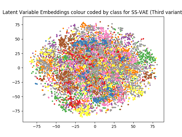
Latent Space Visualization

Figure 5: Latent space embedding for variant 3 with 3000 supervised examples

We use T-SNE to reduce the dimensionality of the latent $\mathbf{z}$ from $50$ to $2$ and visualize the 10 digit classes in Figure 5. Note that the structure of the embedding is quite different than that in the VAE case, where the digits are clearly separated from one another in the embedding. This make sense, since for the semi-supervised case the latent $\mathbf{z}$ is free to use its representational capacity to model, e.g., handwriting style, since the variation between digits is provided by the (partially observed) labels.

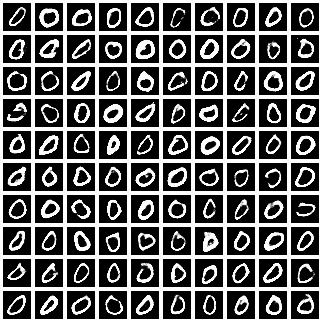
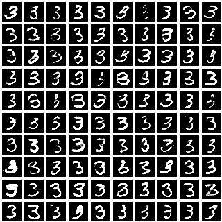
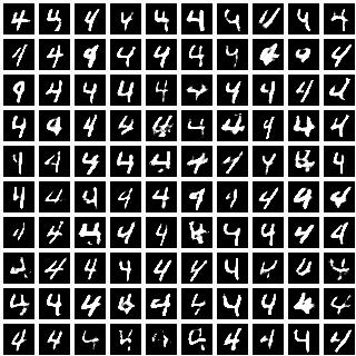
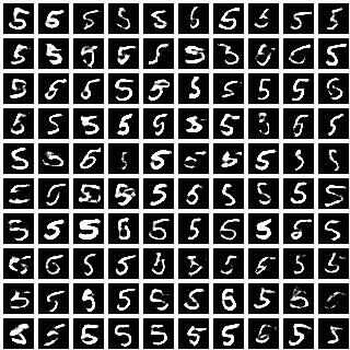
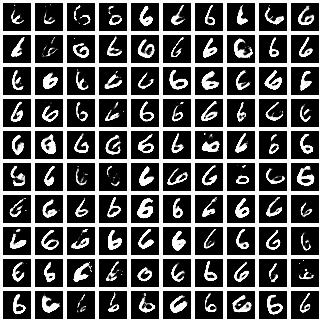
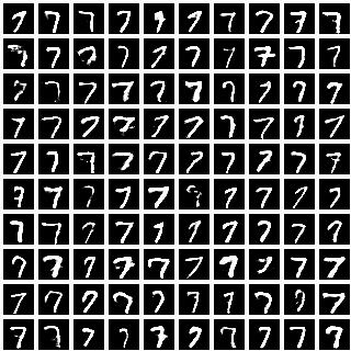
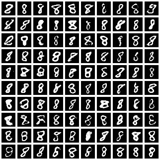
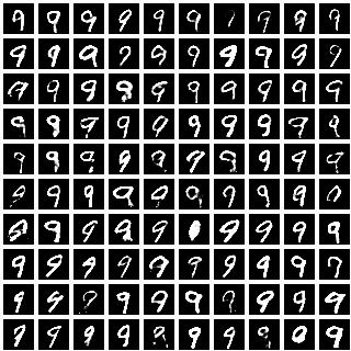
Conditional image generation

Figure 6: Conditional samples obtained by fixing the class label and varying z (for variant 3 with 3000 supervised examples)

We sampled $100$ images for each class label ($0$ to $9$) by sampling different values of the latent variable $\mathbf{z}$. The diversity of handwriting styles exhibited by each digit is consistent with what we saw in the T-SNE visualization, suggesting that the representation learned by $\mathbf{z}$ is disentangled from the class labels.

Final thoughts

We’ve seen that generative models offer a natural approach to semi-supervised machine learning. One of the most attractive features of generative models is that we can explore a large variety of models in a single unified setting. In this tutorial we’ve only been able to explore a small fraction of the possible model and inference setups that are possible. There is no reason to expect that one variant is best; depending on the dataset and application, there will be reason to prefer one over another. And there are a lot of variants (see Figure 7)!

Figure 7: A zoo of semi-supervised generative models

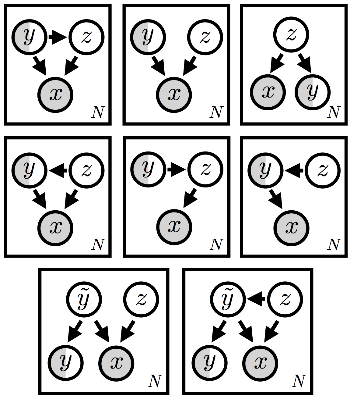
Some of these variants clearly make more sense than others, but a priori it’s difficult to know which ones are worth trying out. This is especially true once we open the door to more complicated setups, like the two models at the bottom of the figure, which include an always latent random variable $\tilde{\mathbf{y}}$ in addition to the partially observed label $\mathbf{y}$. (Incidentally, this class of models—see reference [2] for similar variants—offers another potential solution to the ‘no training’ problem that we identified above.)

The reader probably doesn’t need any convincing that a systematic exploration of even a fraction of these options would be incredibly time-consuming and error-prone if each model and each inference procedure were coded up by scratch. It’s only with the modularity and abstraction made possible by a probabilistic programming system that we can hope to explore the landscape of generative models with any kind of nimbleness—and reap any awaiting rewards.

See the full code on Github.

References

[1] Semi-supervised Learning with Deep Generative Models,     Diederik P. Kingma, Danilo J. Rezende, Shakir Mohamed, Max Welling

[2] Learning Disentangled Representations with Semi-Supervised Deep Generative Models,      N. Siddharth, Brooks Paige, Jan-Willem Van de Meent, Alban Desmaison, Frank Wood,      Noah D. Goodman, Pushmeet Kohli, Philip H.S. Torr