Example: Utilizing Predictive and Deterministic with MCMC and SVI

In this short tutorial we’ll see how to use deterministic statements inside a model and inspect its samples with Predictive class. Additionally a GammaPoisson distribution will be discussed as it’ll be used within our model.

Check out other tutorials that use Predictive and Deterministic:

• Example: analyzing baseball stats with MCMC

• Bayesian Regression - Inference Algorithms (Part 2)

import matplotlib.pyplot as plt
import numpy as np
import pandas as pd
from sklearn.datasets import make_regression
import pyro.distributions as dist
from pyro.infer import MCMC, NUTS, Predictive
from pyro.infer.mcmc.util import summary
from pyro.distributions import constraints
import pyro
import torch

pyro.set_rng_seed(101)

%matplotlib inline
%config InlineBackend.figure_format='retina'

Data generation

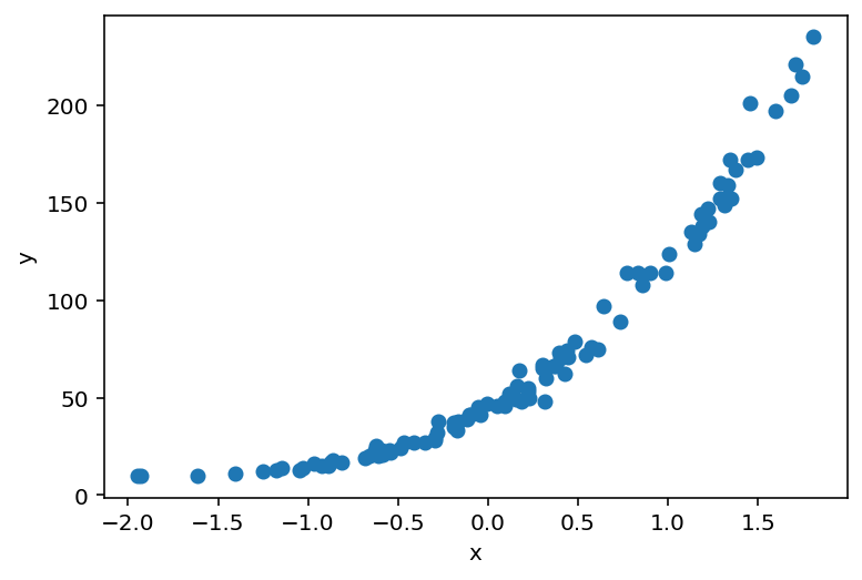
Let’s generate our data with sklearn.datasets.make_regression method where we can determine the number of features, bias and noise power. Also we’ll transform the target variable and make it a torch tensor.

X, y = make_regression(n_features=1, bias=150., noise=5., random_state=108)

X_ = torch.tensor(X, dtype=torch.float)
y_ = torch.tensor((y**3)/100000. + 10., dtype=torch.float)
y_.round_().clamp_(min=0);

plt.scatter(X_, y_)
plt.ylabel('y')
plt.xlabel('x');

Model definition

In our model we first sample coefficient from a normal distribution with zero mean and sampled standard deviation. We use to_event(1) to move the expanded dimension from batch_shape to event_shape as we want to sample from a multivariate normal distribution. deterministic part is used to register a name whose value is fully determined by arguments passed to it. Here we use softplus to be sure that the resulting rate isn’t negative. Then we use vectorized version of plate to record counts from passed dataset as they were sampled from GammaPoisson distribution.

For now this model might be a little obscure but later we will dive into sampled data to better grasp it’s internals.

def model(features, counts):
    N, P = features.shape
    scale = pyro.sample("scale", dist.LogNormal(0, 1))
    coef = pyro.sample("coef", dist.Normal(0, scale).expand([P]).to_event(1))
    rate = pyro.deterministic("rate", torch.nn.functional.softplus(coef @ features.T))
    concentration = pyro.sample("concentration", dist.LogNormal(0, 1))
    with pyro.plate("bins", N):
        return pyro.sample("counts", dist.GammaPoisson(concentration, rate), obs=counts)

Inference

Inference will be done with MCMC algorithm. IMPORTANT! Please note that only scale and coef variables are returned in samples dict. deterministic parts are available via Predictive, similarly as observed samples.

nuts_kernel = NUTS(model)
mcmc = MCMC(nuts_kernel, num_samples=500)

%%time

mcmc.run(X_, y_);

Sample: 100%|██████████| 1000/1000 [00:23, 43.11it/s, step size=6.57e-01, acc. prob=0.922]

CPU times: user 22.8 s, sys: 254 ms, total: 23 s
Wall time: 23.2 s

samples = mcmc.get_samples()
for k, v in samples.items():
    print(f"{k}: {tuple(v.shape)}")

coef: (500, 1)
concentration: (500,)
scale: (500,)

predictive = Predictive(model, samples)(X_, None)
for k, v in predictive.items():
    print(f"{k}: {tuple(v.shape)}")

counts: (500, 100)
rate: (500, 1, 100)

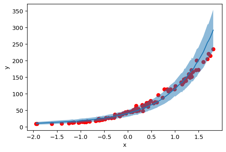
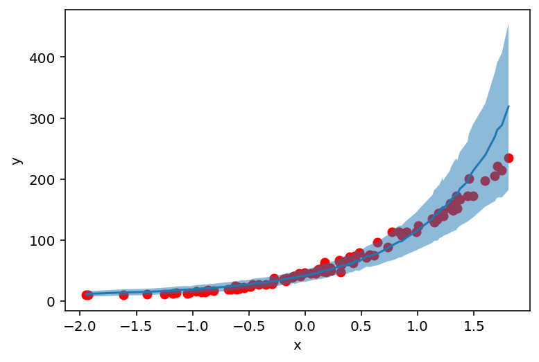
After sampling let’s see how well our model fits the data. We compute sampled counts mean and standard deviation and plot it against the original data.

def prepare_counts_df(predictive):
    counts = predictive['counts'].numpy()
    counts_mean = counts.mean(axis=0)
    counts_std = counts.std(axis=0)

    counts_df = pd.DataFrame({
    "feat": X_.squeeze(),
    "mean": counts_mean,
    "high": counts_mean + counts_std,
    "low": counts_mean - counts_std,
    })

    return counts_df.sort_values(by=['feat'])

counts_df = prepare_counts_df(predictive)

plt.scatter(X_, y_, c='r')
plt.ylabel('y')
plt.xlabel('x')
plt.plot(counts_df['feat'], counts_df['mean'])
plt.fill_between(counts_df['feat'], counts_df['high'], counts_df['low'], alpha=0.5);

But where do these values (and uncertainty) come from? Let’s find out!

Inspecting deterministic part

Now let’s move to the essence of this tutorial. GammaPoisson distribution used here and parameterized with (concentration, rate) arguments is basically an alternative parametrization of NegativeBinomial distribution.

NegativeBinomial answers a question: How many successes will we record before seeing r failures (overall) if each trial wins with probability p?

The reparametrization occurs as follows:

• concentration = r

• rate = 1 / (p + 1)

First we check sampled mean of concentration and coef variables…

print('Concentration mean: ', samples['concentration'].mean().item())
print('Concentration std: ', samples['concentration'].std().item())

Concentration mean:  28.77524757385254
Concentration std:  0.7892239689826965

print('Coef mean: ', samples['coef'].mean().item())
print('Coef std: ', samples['coef'].std().item())

Coef mean:  -1.2473742961883545
Coef std:  0.036095619201660156

…and do reparametrization (again please note that we get it from predictive!).

rates = predictive['rate'].squeeze()
rates_reparam = 1. / (rates + 1.) # here's reparametrization

Now we plot reparametrized rate:

fig, (ax1, ax2) = plt.subplots(1, 2)
fig.set_size_inches(13, 4)

ax1.scatter(X_, rates_reparam.mean(axis=0))
ax1.set_ylabel('mean')
ax1.set_xlabel('x')
ax1.set_title('rate means')
ax2.scatter(X_, rates_reparam.std(axis=0))
ax2.set_ylabel('std')
ax2.set_xlabel('x')
ax2.set_title('rate stds');

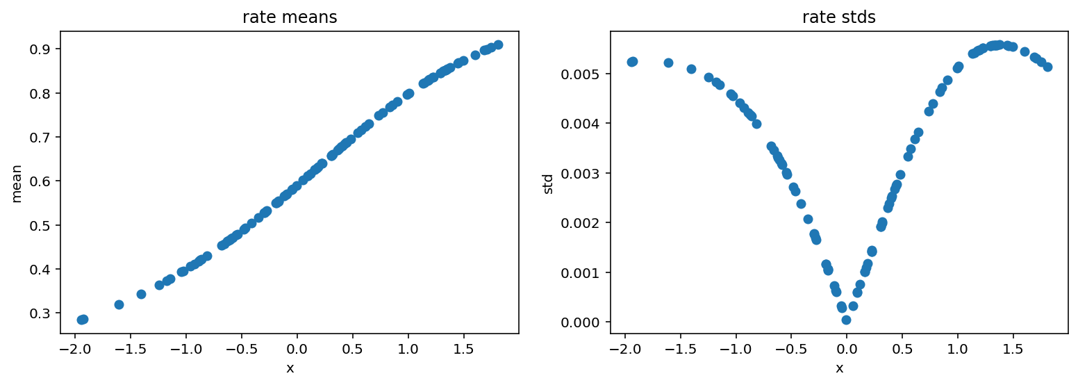
We see that the probability of success rises with x. This means that it will take more and more trials before we observe those 28 failures imposed by concentration parameter.

Intuitively if we want to record 28 failures where each failure occurs with probability 0.5 then it should also take 28 successes. Let’s check if our model follows this logic:

fig, (ax1, ax2) = plt.subplots(1, 2)
fig.set_size_inches(13, 4)

ax1.scatter(X_, y_, c='r')
ax1.plot(counts_df['feat'], counts_df['mean'])
ax1.fill_between(counts_df['feat'], counts_df['high'], counts_df['low'], alpha=0.5)
ax1.axhline(samples['concentration'].mean().item(), c='g', linestyle='dashed')
ax1.axvline(-0.46, c='g', linestyle='dashed')
ax1.set_ylabel('y')
ax1.set_xlabel('x')
ax1.set_title('fitted model')
ax2.scatter(X_, rates_reparam.mean(axis=0))
ax2.axhline(0.5, c='g', linestyle='dashed')
ax2.axvline(-0.46, c='g', linestyle='dashed')
ax2.set_ylabel('mean')
ax2.set_xlabel('x')
ax2.set_title('rate means');

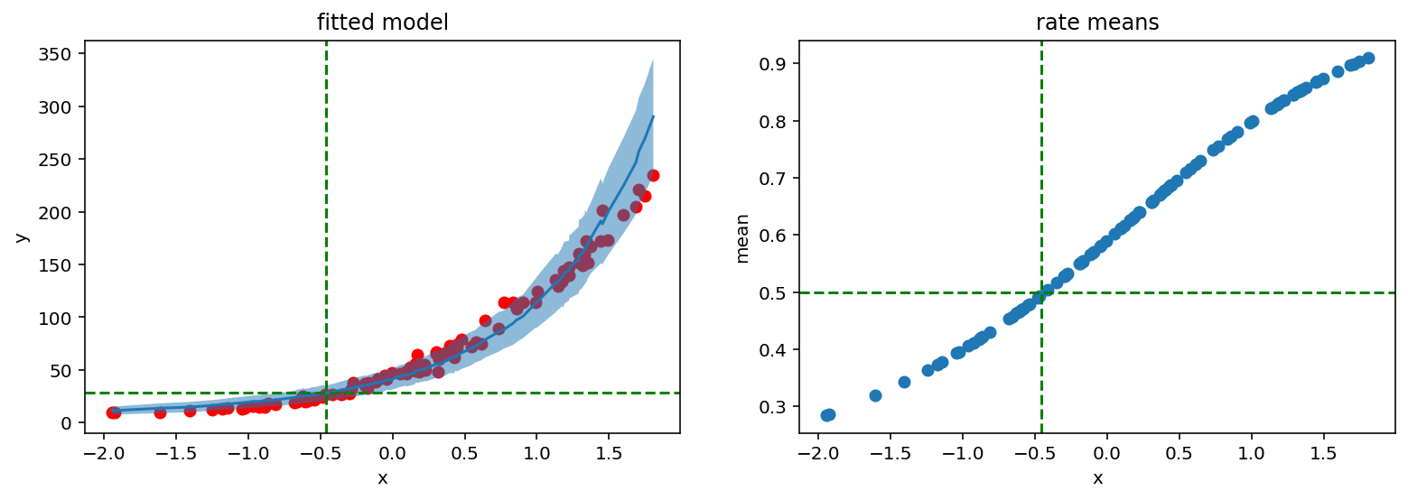
It indeed does. Red lines show that 28 successes and rate 0.5 are located with the same x argument.

SVI approach

Predictive class can also be used with the SVI method. In the next section we will use it with AutoGuide’s guide and manually designed one.

from pyro.infer import SVI, Trace_ELBO
from pyro.optim import Adam
from pyro.infer.autoguide import AutoNormal

Manually defined guide

First we define our guide with all sample sites that are present in the model and parametrize them with learnable parameters. Then we perform gradient descent with Adam optimizer.

def guide(features, counts):
    N, P = features.shape

    scale_param = pyro.param("scale_param", torch.tensor(0.1), constraint=constraints.positive)
    loc_param = pyro.param("loc_param", torch.tensor(0.0))
    scale = pyro.sample("scale", dist.Delta(scale_param))
    coef = pyro.sample("coef", dist.Normal(loc_param, scale).expand([P]).to_event(1))

    concentration_param = pyro.param("concentration_param", torch.tensor(0.1), constraint=constraints.positive)
    concentration = pyro.sample("concentration", dist.Delta(concentration_param))

pyro.clear_param_store()

adam_params = {"lr": 0.005, "betas": (0.90, 0.999)}
optimizer = Adam(adam_params)

svi = SVI(model, guide, optimizer, loss=Trace_ELBO())

%%time

n_steps = 5001

for step in range(n_steps):
    loss = svi.step(X_, y_)
    if step % 1000 == 0:
        print('Loss: ', loss)

Loss:  4509.724546432495
Loss:  410.72651755809784
Loss:  417.1552972793579
Loss:  395.92131960392
Loss:  447.41201531887054
Loss:  445.11494612693787
CPU times: user 21.2 s, sys: 73.4 ms, total: 21.2 s
Wall time: 21.3 s

Pyros parameter store is comprised of learned parameters that will be used in Predictive stage. Instead of providing samples we pass guide parameter to construct predictive distribution.

list(pyro.get_param_store().items())

[('scale_param', tensor(0.1965, grad_fn=<AddBackward0>)),
 ('loc_param', tensor(-1.2427, requires_grad=True)),
 ('concentration_param', tensor(29.1642, grad_fn=<AddBackward0>))]

predictive_svi = Predictive(model, guide=guide, num_samples=500)(X_, None)
for k, v in predictive_svi.items():
    print(f"{k}: {tuple(v.shape)}")

scale: (500, 1)
coef: (500, 1, 1)
concentration: (500, 1)
counts: (500, 100)
rate: (500, 1, 100)

counts_df = prepare_counts_df(predictive_svi)

plt.scatter(X_, y_, c='r')
plt.ylabel('y')
plt.xlabel('x')
plt.plot(counts_df['feat'], counts_df['mean'])
plt.fill_between(counts_df['feat'], counts_df['high'], counts_df['low'], alpha=0.5);

AutoGuide

Another approach for conducting SVI is to rely on automatic guide generation. Here we use AutoNormal that underneath uses a normal distribution with a diagonal covariance matrix.

pyro.clear_param_store()

adam_params = {"lr": 0.005, "betas": (0.90, 0.999)}
optimizer = Adam(adam_params)

auto_guide = AutoNormal(model)

svi = SVI(model, auto_guide, optimizer, loss=Trace_ELBO())

%%time

n_steps = 3001

for step in range(n_steps):
    loss = svi.step(X_, y_)
    if step % 1000 == 0:
        print('Loss: ', loss)

Loss:  3881.8888041973114
Loss:  380.9036132991314
Loss:  375.7684025168419
Loss:  377.94497936964035
CPU times: user 18.8 s, sys: 83.8 ms, total: 18.9 s
Wall time: 19 s

auto_guide(X_, y_)

{'scale': tensor(1.9367, grad_fn=<ExpandBackward>),
 'coef': tensor([-1.2498], grad_fn=<ExpandBackward>),
 'concentration': tensor(29.5432, grad_fn=<ExpandBackward>)}

As we check PARAM_STORE we see that each sample site is approximated with a normal distribution.

list(pyro.get_param_store().items())

[('AutoNormal.locs.scale',
  Parameter containing:
  tensor(0.3204, requires_grad=True)),
 ('AutoNormal.scales.scale', tensor(0.5149, grad_fn=<SoftplusBackward>)),
 ('AutoNormal.locs.coef',
  Parameter containing:
  tensor([-1.2510], requires_grad=True)),
 ('AutoNormal.scales.coef', tensor([0.0413], grad_fn=<SoftplusBackward>)),
 ('AutoNormal.locs.concentration',
  Parameter containing:
  tensor(3.3640, requires_grad=True)),
 ('AutoNormal.scales.concentration',
  tensor(0.0299, grad_fn=<SoftplusBackward>))]

Finally we again construct a predictive distribution and plot counts. For all three methods we managed to get similar results for our parameters.

predictive_svi = Predictive(model, guide=auto_guide, num_samples=500)(X_, None)
for k, v in predictive_svi.items():
    print(f"{k}: {tuple(v.shape)}")

scale: (500, 1)
coef: (500, 1, 1)
concentration: (500, 1)
counts: (500, 100)
rate: (500, 1, 100)

counts_df = prepare_counts_df(predictive_svi)

plt.scatter(X_, y_, c='r')
plt.ylabel('y')
plt.xlabel('x')
plt.plot(counts_df['feat'], counts_df['mean'])
plt.fill_between(counts_df['feat'], counts_df['high'], counts_df['low'], alpha=0.5);