Forecasting III: hierarchical models

This tutorial covers hierarchical multivariate time series modeling with the pyro.contrib.forecast module. This tutorial assumes the reader is already familiar with SVI, tensor shapes, and univariate forecasting.

See also:

• Forecasting I: univariate, heavy tailed

• Forecasting II: state space models

Summary

• Hierarchial forecasting works like any other hierarchial modeling in Pyro.

• To create hierarchical models in Pyro, use the plate context manager.

• To subsample data during training, pass a create_plates() callback to the Forecaster.

• You can subsample time series, but you can’t subsample the time_plate.

import math
import torch
import pyro
import pyro.distributions as dist
import pyro.poutine as poutine
from pyro.contrib.examples.bart import load_bart_od
from pyro.contrib.forecast import ForecastingModel, Forecaster, eval_crps
from pyro.infer.reparam import LocScaleReparam, SymmetricStableReparam
from pyro.ops.tensor_utils import periodic_repeat
from pyro.ops.stats import quantile
import matplotlib.pyplot as plt

%matplotlib inline
assert pyro.__version__.startswith('1.9.1')
pyro.set_rng_seed(20200305)

Let’s again look at the BART train ridership dataset:

dataset = load_bart_od()
print(dataset.keys())
print(dataset["counts"].shape)
print(" ".join(dataset["stations"]))

dict_keys(['stations', 'start_date', 'counts'])
torch.Size([78888, 50, 50])
12TH 16TH 19TH 24TH ANTC ASHB BALB BAYF BERY CAST CIVC COLM COLS CONC DALY DBRK DELN DUBL EMBR FRMT FTVL GLEN HAYW LAFY LAKE MCAR MLBR MLPT MONT NBRK NCON OAKL ORIN PCTR PHIL PITT PLZA POWL RICH ROCK SANL SBRN SFIA SHAY SSAN UCTY WARM WCRK WDUB WOAK

Multivariate time series

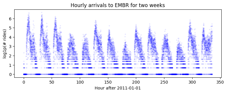
Let’s start by modeling arrivals to Embarcadero station, from each of the other 50 stations. Note this is nine years of hourly data, so the dataset is quite long.

T, O, D = dataset["counts"].shape
data = dataset["counts"][:, :, dataset["stations"].index("EMBR")].log1p()
print(data.shape)
plt.figure(figsize=(9, 3))
plt.plot(data[-24 * 7 * 2:], 'b.', alpha=0.1, markeredgewidth=0)
plt.title("Hourly arrivals to EMBR for two weeks")
plt.ylabel("log1p(# rides)")
plt.xlabel("Hour after 2011-01-01");

torch.Size([78888, 50])

Let’s try a two-component model with series-local level + series-local seasonality.

class Model1(ForecastingModel):
    def model(self, zero_data, covariates):
        duration, data_dim = zero_data.shape

        # Let's model each time series as a Levy stable process, and share process parameters
        # across time series. To do that in Pyro, we'll declare the shared random variables
        # outside of the "origin" plate:
        drift_stability = pyro.sample("drift_stability", dist.Uniform(1, 2))
        drift_scale = pyro.sample("drift_scale", dist.LogNormal(-20, 5))
        with pyro.plate("origin", data_dim, dim=-2):
            # Now inside of the origin plate we sample drift and seasonal components.
            # All the time series inside the "origin" plate are independent,
            # given the drift parameters above.
            with self.time_plate:
                # We combine two different reparameterizers: the inner SymmetricStableReparam
                # is needed for the Stable site, and the outer LocScaleReparam is optional but
                # appears to improve inference.
                with poutine.reparam(config={"drift": LocScaleReparam()}):
                    with poutine.reparam(config={"drift": SymmetricStableReparam()}):
                        drift = pyro.sample("drift",
                                            dist.Stable(drift_stability, 0, drift_scale))

            with pyro.plate("hour_of_week", 24 * 7, dim=-1):
                seasonal = pyro.sample("seasonal", dist.Normal(0, 5))

        # Now outside of the time plate we can perform time-dependent operations like
        # integrating over time. This allows us to create a motion with slow drift.
        seasonal = periodic_repeat(seasonal, duration, dim=-1)
        motion = drift.cumsum(dim=-1)  # A Levy stable motion to model shocks.
        prediction = motion + seasonal

        # Next we do some reshaping. Pyro's forecasting framework assumes all data is
        # multivariate of shape (duration, data_dim), but the above code uses an "origins"
        # plate that is left of the time_plate. Our prediction starts off with shape
        assert prediction.shape[-2:] == (data_dim, duration)
        # We need to swap those dimensions but keep the -2 dimension intact, in case Pyro
        # adds sample dimensions to the left of that.
        prediction = prediction.unsqueeze(-1).transpose(-1, -3)
        assert prediction.shape[-3:] == (1, duration, data_dim), prediction.shape

        # Finally we can construct a noise distribution.
        # We will share parameters across all time series.
        obs_scale = pyro.sample("obs_scale", dist.LogNormal(-5, 5))
        noise_dist = dist.Normal(0, obs_scale.unsqueeze(-1))
        self.predict(noise_dist, prediction)

Now let’s split data into train and test. This is a bigger dataset, so we’ll train on only 90 days of data.

T2 = data.size(-2)    # end
T1 = T2 - 24 * 7 * 2  # train/test split
T0 = T1 - 24 * 90     # beginning: train on 90 days of data
covariates = torch.zeros(data.size(-2), 0)  # empty covariates

%%time
pyro.set_rng_seed(1)
pyro.clear_param_store()
covariates = torch.zeros(len(data), 0)  # empty
forecaster = Forecaster(Model1(), data[T0:T1], covariates[T0:T1],
                        learning_rate=0.1, num_steps=501, log_every=50)
for name, value in forecaster.guide.median().items():
    if value.numel() == 1:
        print("{} = {:0.4g}".format(name, value.item()))

INFO     step    0 loss = 705188
INFO     step   50 loss = 7.7227
INFO     step  100 loss = 3.44737
INFO     step  150 loss = 1.98431
INFO     step  200 loss = 1.48724
INFO     step  250 loss = 1.25238
INFO     step  300 loss = 1.18827
INFO     step  350 loss = 1.12238
INFO     step  400 loss = 1.10252
INFO     step  450 loss = 1.07717
INFO     step  500 loss = 1.05626

drift_stability = 1.997
drift_scale = 3.863e-08
obs_scale = 0.4636
CPU times: user 28.1 s, sys: 4.29 s, total: 32.4 s
Wall time: 31.9 s

samples = forecaster(data[T0:T1], covariates[T0:T2], num_samples=100)
samples.clamp_(min=0)  # apply domain knowledge: the samples must be positive
p10, p50, p90 = quantile(samples[:, 0], (0.1, 0.5, 0.9)).squeeze(-1)
crps = eval_crps(samples, data[T1:T2])
print(samples.shape, p10.shape)

fig, axes = plt.subplots(8, 1, figsize=(9, 10), sharex=True)
plt.subplots_adjust(hspace=0)
axes[0].set_title("log1p(# hourly arrivals to EMBR) (CRPS = {:0.3g})".format(crps))
for i, ax in enumerate(axes):
    ax.axvline(78736, color="green", lw=20, alpha=0.2)
    ax.fill_between(torch.arange(T1, T2), p10[:, i], p90[:, i], color="red", alpha=0.3)
    ax.plot(torch.arange(T1, T2), p50[:, i], 'r-', lw=1, label='forecast')
    ax.plot(torch.arange(T1 - 24 * 7, T2),
            data[T1 - 24 * 7: T2, i], 'k-', lw=1, label='truth')
    ax.set_ylabel("from {}".format(dataset["stations"][i]))
ax.set_xlabel("Hour after 2011-01-01")
ax.text(78732, -3, "Christmas", color="green", horizontalalignment="center")
ax.set_xlim(T1 - 24 * 7, T2)
axes[0].legend(loc="best");

torch.Size([100, 1, 336, 50]) torch.Size([336, 50])

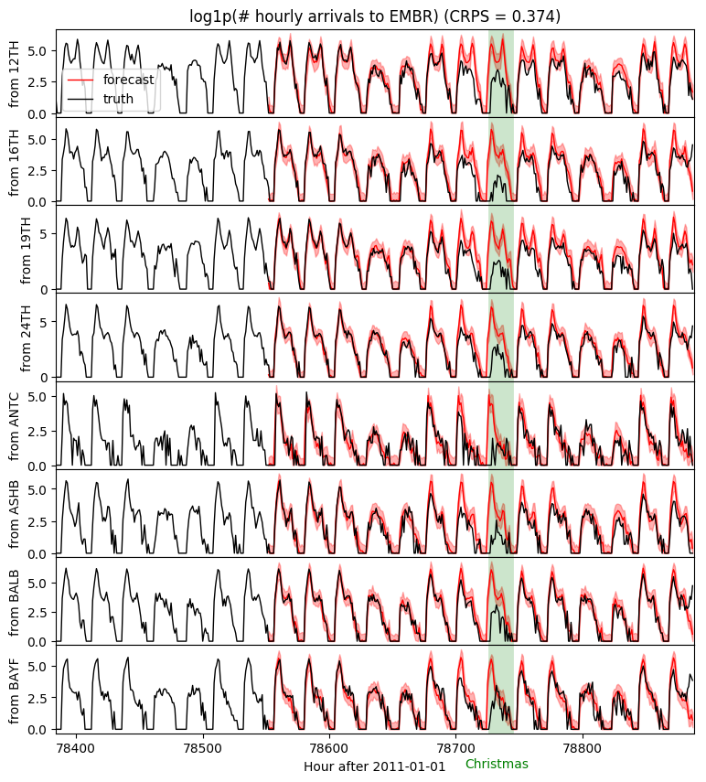
Note the poor predictions on the Christmas holiday. This is to be expected since we only trained on 90 days of data and have not modeled holidays. To accurately forecast holiday behavior we would need to train on multiple years of data, include yearly seasonality components, and ideally include holiday features in covariates.

Deeper hierarchical models

Next let’s consider a larger hierarchy: all 50 x 50 = 2500 pairs of stations.

data = dataset["counts"].permute(1, 2, 0).unsqueeze(-1).log1p().contiguous()
print(dataset["counts"].shape, data.shape)

torch.Size([78888, 50, 50]) torch.Size([50, 50, 78888, 1])

This model will have three levels of hierarchy: origin, destination, and time, each modeled as a plate. We can create sample sites in many combinations of plate contexts, allowing many different ways to share statistical strength.

class Model2(ForecastingModel):
    def model(self, zero_data, covariates):
        num_stations, num_stations, duration, one = zero_data.shape

        # We construct plates once so we can reuse them later. We ensure they don't collide by
        # specifying different dim args for each: -3, -2, -1. Note the time_plate is dim=-1.
        origin_plate = pyro.plate("origin", num_stations, dim=-3)
        destin_plate = pyro.plate("destin", num_stations, dim=-2)
        hour_of_week_plate = pyro.plate("hour_of_week", 24 * 7, dim=-1)

        # Let's model the time-dependent part with only O(num_stations * duration) many
        # parameters, rather than the full possible O(num_stations ** 2 * duration) data size.
        drift_stability = pyro.sample("drift_stability", dist.Uniform(1, 2))
        drift_scale = pyro.sample("drift_scale", dist.LogNormal(-20, 5))
        with origin_plate:
            with hour_of_week_plate:
                origin_seasonal = pyro.sample("origin_seasonal", dist.Normal(0, 5))
        with destin_plate:
            with hour_of_week_plate:
                destin_seasonal = pyro.sample("destin_seasonal", dist.Normal(0, 5))
            with self.time_plate:
                with poutine.reparam(config={"drift": LocScaleReparam()}):
                    with poutine.reparam(config={"drift": SymmetricStableReparam()}):
                        drift = pyro.sample("drift",
                                            dist.Stable(drift_stability, 0, drift_scale))
        # Additionally we can model a static pairwise station->station affinity, which e.g.
        # can compensate for the fact that people tend not to travel from a station to itself.
        with origin_plate, destin_plate:
            pairwise = pyro.sample("pairwise", dist.Normal(0, 1))

        # Outside of the time plate we can now form the prediction.
        seasonal = origin_seasonal + destin_seasonal  # Note this broadcasts.
        seasonal = periodic_repeat(seasonal, duration, dim=-1)
        motion = drift.cumsum(dim=-1)  # A Levy stable motion to model shocks.
        prediction = motion + seasonal + pairwise

        # We will decompose the noise scale parameter into
        # an origin-local and a destination-local component.
        with origin_plate:
            origin_scale = pyro.sample("origin_scale", dist.LogNormal(-5, 5))
        with destin_plate:
            destin_scale = pyro.sample("destin_scale", dist.LogNormal(-5, 5))
        scale = origin_scale + destin_scale

        # At this point our prediction and scale have shape (50, 50, duration) and (50, 50, 1)
        # respectively, but we want them to have shape (50, 50, duration, 1) to satisfy the
        # Forecaster requirements.
        scale = scale.unsqueeze(-1)
        prediction = prediction.unsqueeze(-1)

        # Finally we construct a noise distribution and call the .predict() method.
        # Note that predict must be called inside the origin and destination plates.
        noise_dist = dist.Normal(0, scale)
        with origin_plate, destin_plate:
            self.predict(noise_dist, prediction)

%%time
pyro.set_rng_seed(1)
pyro.clear_param_store()
covariates = torch.zeros(data.size(-2), 0)  # empty
forecaster = Forecaster(Model2(), data[..., T0:T1, :], covariates[T0:T1],
                        learning_rate=0.1, learning_rate_decay=1, num_steps=501, log_every=50)
for name, value in forecaster.guide.median().items():
    if value.numel() == 1:
        print("{} = {:0.4g}".format(name, value.item()))

INFO     step    0 loss = 4.83016e+10
INFO     step   50 loss = 133310
INFO     step  100 loss = 2.26326
INFO     step  150 loss = 0.879302
INFO     step  200 loss = 0.948082
INFO     step  250 loss = 0.897158
INFO     step  300 loss = 1.43375
INFO     step  350 loss = 0.700097
INFO     step  400 loss = 0.693259
INFO     step  450 loss = 0.691785
INFO     step  500 loss = 0.695014

drift_stability = 1.593
drift_scale = 6.594e-07
CPU times: user 2min 9s, sys: 54.6 s, total: 3min 3s
Wall time: 3min 4s

Now we can forecast forward entire joint samples of every origin-destination-time triple. The output of forecast(...) will have shape (num_samples, num_stations, num_stations, duration, 1). The trailing 1 just means that we are modeling this as a batch of univariate time series (although with hierarchical coupling).

%%time
samples = forecaster(data[..., T0:T1, :], covariates[T0:T2], num_samples=100)
samples.clamp_(min=0)  # apply domain knowledge: the samples must be positive
p10, p50, p90 = quantile(samples[..., 0], (0.1, 0.5, 0.9))
crps = eval_crps(samples, data[..., T1:T2, :])
print(samples.shape, p10.shape)

torch.Size([100, 50, 50, 336, 1]) torch.Size([50, 50, 336])
CPU times: user 21.5 s, sys: 7.95 s, total: 29.4 s
Wall time: 32.4 s

Now we can examine forecasts for any station-station pair. Let’s look at Antioch, one of the newer stations with least volume.

fig, axes = plt.subplots(8, 1, figsize=(9, 10), sharex=True)
plt.subplots_adjust(hspace=0)
j = dataset["stations"].index("ANTC")
axes[0].set_title("log1p(# hourly arrivals to ANTC) (CRPS = {:0.3g})".format(crps))
for i, ax in enumerate(axes):
    ax.axvline(78736, color="green", lw=20, alpha=0.2)
    ax.fill_between(torch.arange(T1, T2), p10[i, j], p90[i, j], color="red", alpha=0.3)
    ax.plot(torch.arange(T1, T2), p50[i, j], 'r-', lw=1, label='forecast')
    ax.plot(torch.arange(T1 - 24 * 7, T2),
            data[i, j, T1 - 24 * 7: T2, 0], 'k-', lw=1, label='truth')
    ax.set_ylabel("from {}".format(dataset["stations"][i]))
ax.set_xlabel("Hour after 2011-01-01")
ax.text(78732, -0.8, "Christmas", color="green", horizontalalignment="center")
ax.set_xlim(T1 - 24 * 7, T2)
axes[0].legend(loc="best");

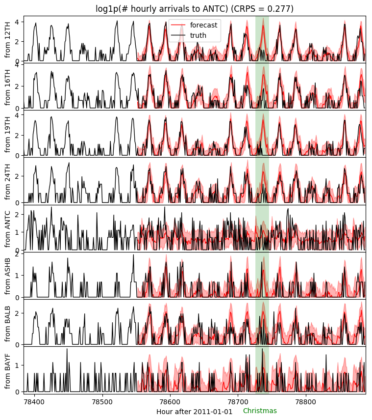
Notice that the hierarchy allows the model to make accurate predictions even for very low-volume (station,station) pairs. For example almost nobody rides from Ashby station to Antioch.

Subsampling

It can be expensive to train models of high-dimensional time series data. However since we’re using stochastic variational inference for training, we can subsample some of the data plates, trading gradient variance for speed. In our BART example we can subsample both origins and destinations (but we can never subsample the time_plate).

To enable subampling in a Forecaster (or more generally in any Pyro AutoDelta or Autonormal guide), we need to define a callback fuction that creates subsampled plates in the guide. This callback will be named create_plates(). It will input the same (zero_data, covariates) args as the model (or more generally the same (*args, **kwargs)), and will return a plate or iterable of plates.

Let’s define a create_plates() callback that subsamples both the “origin” plate and the “destin” plate to 20% of their data, resulting in only 4% of data being touched each iteration.

def create_plates(zero_data, covariates):
    num_origins, num_destins, duration, one = zero_data.shape
    return [pyro.plate("origin", num_origins, subsample_size=10, dim=-3),
            pyro.plate("destin", num_destins, subsample_size=10, dim=-2)]

Now we can train as usual. However since gradient estimates will have higher variance, we run for more iterations. We’ll use the same learning rate and let the Adam optimizer adjust per-parameter learning rates.

%%time
pyro.set_rng_seed(1)
pyro.clear_param_store()
covariates = torch.zeros(data.size(-2), 0)  # empty
forecaster = Forecaster(Model2(), data[..., T0:T1, :], covariates[T0:T1],
                        create_plates=create_plates,
                        learning_rate=0.1, num_steps=1201, log_every=50)
for name, value in forecaster.guide.median().items():
    if value.numel() == 1:
        print("{} = {:0.4g}".format(name, value.item()))

INFO     step    0 loss = 58519
INFO     step   50 loss = 3.61814e+09
INFO     step  100 loss = 965.526
INFO     step  150 loss = 9000.55
INFO     step  200 loss = 1003.25
INFO     step  250 loss = 31.0245
INFO     step  300 loss = 1.53046
INFO     step  350 loss = 1.22161
INFO     step  400 loss = 0.991503
INFO     step  450 loss = 0.79876
INFO     step  500 loss = 0.83428
INFO     step  550 loss = 0.804639
INFO     step  600 loss = 0.686404
INFO     step  650 loss = 0.803543
INFO     step  700 loss = 0.783584
INFO     step  750 loss = 0.618151
INFO     step  800 loss = 0.772374
INFO     step  850 loss = 0.684863
INFO     step  900 loss = 0.77464
INFO     step  950 loss = 0.862912
INFO     step 1000 loss = 0.74513
INFO     step 1050 loss = 0.756743
INFO     step 1100 loss = 0.772813
INFO     step 1150 loss = 0.68757
INFO     step 1200 loss = 0.778757

drift_stability = 1.502
drift_scale = 4.265e-07
CPU times: user 46.2 s, sys: 7.11 s, total: 53.3 s
Wall time: 52.9 s

Even though we’re running for more iterations (1201 instead of 501), each iteration is cheaper, and the total time is reduced by more than a factor of three, with nearly identical accuracy:

%%time
samples = forecaster(data[..., T0:T1, :], covariates[T0:T2], num_samples=100)
samples.clamp_(min=0)  # apply domain knowledge: the samples must be positive
crps = eval_crps(samples, data[..., T1:T2, :])
print("CRPS = {:0.4g}".format(crps))

CRPS = 0.2792
CPU times: user 14.6 s, sys: 5.77 s, total: 20.4 s
Wall time: 23.1 s