Bayesian Regression - Introduction (Part 1)
Regression is one of the most common and basic supervised learning tasks in machine learning. Suppose we’re given a dataset \(\mathcal{D}\) of the form
The goal of linear regression is to fit a function to the data of the form:
where \(w\) and \(b\) are learnable parameters and \(\epsilon\) represents observation noise. Specifically \(w\) is a matrix of weights and \(b\) is a bias vector.
In this tutorial, we will first implement linear regression in PyTorch and learn point estimates for the parameters \(w\) and \(b\). Then we will see how to incorporate uncertainty into our estimates by using Pyro to implement Bayesian regression. Additionally, we will learn how to use the Pyro’s utility functions to do predictions and serve our model using TorchScript.
Tutorial Outline
Setup
Let’s begin by importing the modules we’ll need.
[1]:
%reset -s -f
[2]:
import os
from functools import partial
import torch
import numpy as np
import pandas as pd
import seaborn as sns
import matplotlib.pyplot as plt

import pyro
import pyro.distributions as dist

# for CI testing
smoke_test = ('CI' in os.environ)
assert pyro.__version__.startswith('1.9.1')
pyro.set_rng_seed(1)


# Set matplotlib settings
%matplotlib inline
plt.style.use('default')
Dataset
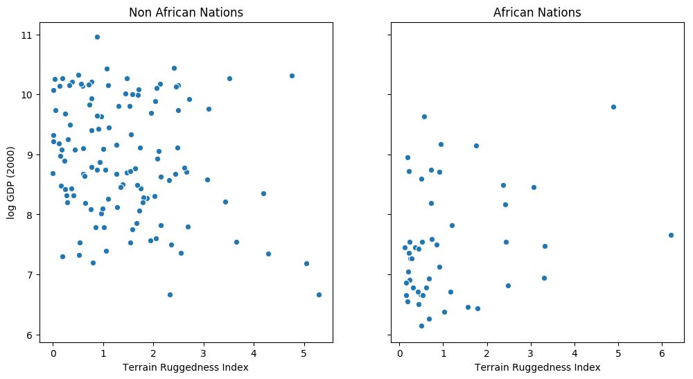
The following example is adapted from [1]. We would like to explore the relationship between topographic heterogeneity of a nation as measured by the Terrain Ruggedness Index (variable rugged in the dataset) and its GDP per capita. In particular, it was noted by the authors in [2] that terrain ruggedness or bad geography is related to poorer economic performance outside of Africa, but rugged terrains have had a reverse effect on income for African nations. Let us look at the data and investigate this relationship. We will be focusing on three features from the dataset:
rugged: quantifies the Terrain Ruggedness Indexcont_africa: whether the given nation is in Africargdppc_2000: Real GDP per capita for the year 2000
The response variable GDP is highly skewed, so we will log-transform it.
[3]:
DATA_URL = "https://d2hg8soec8ck9v.cloudfront.net/datasets/rugged_data.csv"
data = pd.read_csv(DATA_URL, encoding="ISO-8859-1")
df = data[["cont_africa", "rugged", "rgdppc_2000"]]
df = df[np.isfinite(df.rgdppc_2000)]
df["rgdppc_2000"] = np.log(df["rgdppc_2000"])
[4]:
fig, ax = plt.subplots(nrows=1, ncols=2, figsize=(12, 6), sharey=True)
african_nations = df[df["cont_africa"] == 1]
non_african_nations = df[df["cont_africa"] == 0]
sns.scatterplot(x=non_african_nations["rugged"],
                y=non_african_nations["rgdppc_2000"],
                ax=ax[0])
ax[0].set(xlabel="Terrain Ruggedness Index",
          ylabel="log GDP (2000)",
          title="Non African Nations")
sns.scatterplot(x=african_nations["rugged"],
                y=african_nations["rgdppc_2000"],
                ax=ax[1])
ax[1].set(xlabel="Terrain Ruggedness Index",
          ylabel="log GDP (2000)",
          title="African Nations");
Linear Regression
We would like to predict log GDP per capita of a nation as a function of two features from the dataset - whether the nation is in Africa, and its Terrain Ruggedness Index. We will create a trivial class called PyroModule[nn.Linear] that subclasses PyroModule and torch.nn.Linear. PyroModule is very similar to PyTorch’s nn.Module, but additionally supports Pyro
primitives as attributes that can be modified by Pyro’s effect handlers (see the next section on how we can have module attributes that are pyro.sample primitives). Some general notes:
Learnable parameters in PyTorch modules are instances of
nn.Parameter, in this case theweightandbiasparameters of thenn.Linearclass. When declared inside aPyroModuleas attributes, these are automatically registered in Pyro’s param store. While this model does not require us to constrain the value of these parameters during optimization, this can also be easily achieved inPyroModuleusing the PyroParam statement.Note that while the
forwardmethod ofPyroModule[nn.Linear]inherits fromnn.Linear, it can also be easily overridden. e.g. in the case of logistic regression, we apply a sigmoid transformation to the linear predictor.
[5]:
from torch import nn
from pyro.nn import PyroModule

assert issubclass(PyroModule[nn.Linear], nn.Linear)
assert issubclass(PyroModule[nn.Linear], PyroModule)
Training with PyTorch Optimizers
Note that in addition to the two features rugged and cont_africa, we also include an interaction term in our model, which lets us separately model the effect of ruggedness on the GDP for nations within and outside Africa.
We use the mean squared error (MSE) as our loss and Adam as our optimizer from the torch.optim module. We would like to optimize the parameters of our model, namely the weight and bias parameters of the network, which corresponds to our regression coefficents and the intercept.
[6]:
# Dataset: Add a feature to capture the interaction between "cont_africa" and "rugged"
df["cont_africa_x_rugged"] = df["cont_africa"] * df["rugged"]
data = torch.tensor(df[["cont_africa", "rugged", "cont_africa_x_rugged", "rgdppc_2000"]].values,
                        dtype=torch.float)
x_data, y_data = data[:, :-1], data[:, -1]

# Regression model
linear_reg_model = PyroModule[nn.Linear](3, 1)

# Define loss and optimize
loss_fn = torch.nn.MSELoss(reduction='sum')
optim = torch.optim.Adam(linear_reg_model.parameters(), lr=0.05)
num_iterations = 1500 if not smoke_test else 2

def train():
    # run the model forward on the data
    y_pred = linear_reg_model(x_data).squeeze(-1)
    # calculate the mse loss
    loss = loss_fn(y_pred, y_data)
    # initialize gradients to zero
    optim.zero_grad()
    # backpropagate
    loss.backward()
    # take a gradient step
    optim.step()
    return loss

for j in range(num_iterations):
    loss = train()
    if (j + 1) % 50 == 0:
        print("[iteration %04d] loss: %.4f" % (j + 1, loss.item()))


# Inspect learned parameters
print("Learned parameters:")
for name, param in linear_reg_model.named_parameters():
    print(name, param.data.numpy())
[iteration 0050] loss: 3179.7852
[iteration 0100] loss: 1616.1371
[iteration 0150] loss: 1109.4117
[iteration 0200] loss: 833.7545
[iteration 0250] loss: 637.5822
[iteration 0300] loss: 488.2652
[iteration 0350] loss: 376.4650
[iteration 0400] loss: 296.0483
[iteration 0450] loss: 240.6140
[iteration 0500] loss: 203.9386
[iteration 0550] loss: 180.6171
[iteration 0600] loss: 166.3493
[iteration 0650] loss: 157.9457
[iteration 0700] loss: 153.1786
[iteration 0750] loss: 150.5735
[iteration 0800] loss: 149.2020
[iteration 0850] loss: 148.5065
[iteration 0900] loss: 148.1668
[iteration 0950] loss: 148.0070
[iteration 1000] loss: 147.9347
[iteration 1050] loss: 147.9032
[iteration 1100] loss: 147.8900
[iteration 1150] loss: 147.8847
[iteration 1200] loss: 147.8827
[iteration 1250] loss: 147.8819
[iteration 1300] loss: 147.8817
[iteration 1350] loss: 147.8816
[iteration 1400] loss: 147.8815
[iteration 1450] loss: 147.8815
[iteration 1500] loss: 147.8815
Learned parameters:
weight [[-1.9478593  -0.20278624  0.39330274]]
bias [9.22308]
Plotting the Regression Fit
Let us plot the regression fit for our model, separately for countries outside and within Africa.
[7]:
fit = df.copy()
fit["mean"] = linear_reg_model(x_data).detach().cpu().numpy()

fig, ax = plt.subplots(nrows=1, ncols=2, figsize=(12, 6), sharey=True)
african_nations = fit[fit["cont_africa"] == 1]
non_african_nations = fit[fit["cont_africa"] == 0]
fig.suptitle("Regression Fit", fontsize=16)
ax[0].plot(non_african_nations["rugged"], non_african_nations["rgdppc_2000"], "o")
ax[0].plot(non_african_nations["rugged"], non_african_nations["mean"], linewidth=2)
ax[0].set(xlabel="Terrain Ruggedness Index",
          ylabel="log GDP (2000)",
          title="Non African Nations")
ax[1].plot(african_nations["rugged"], african_nations["rgdppc_2000"], "o")
ax[1].plot(african_nations["rugged"], african_nations["mean"], linewidth=2)
ax[1].set(xlabel="Terrain Ruggedness Index",
          ylabel="log GDP (2000)",
          title="African Nations");
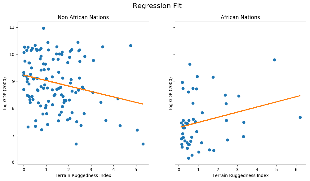
We notice that the relationship between terrain ruggedness has an inverse relationship with GDP for non-African nations, but it positively affects the GDP for African nations. It is however unclear how robust this trend is. In particular, we would like to understand how the regression fit would vary due to parameter uncertainty. To address this, we will build a simple Bayesian model for linear regression. Bayesian modeling offers a systematic framework for reasoning about model uncertainty. Instead of just learning point estimates, we’re going to learn a distribution over parameters that are consistent with the observed data.
Bayesian Regression with Pyro’s Stochastic Variational Inference (SVI)
Model
In order to make our linear regression Bayesian, we need to put priors on the parameters \(w\) and \(b\). These are distributions that represent our prior belief about reasonable values for \(w\) and \(b\) (before observing any data).
Making a Bayesian model for linear regression is very intuitive using PyroModule as earlier. Note the following:
The
BayesianRegressionmodule internally uses the samePyroModule[nn.Linear]module. However, note that we replace theweightand thebiasof the this module withPyroSamplestatements. These statements allow us to place a prior over theweightandbiasparameters, instead of treating them as fixed learnable parameters. For the bias component, we set a reasonably wide prior since it is likely to be substantially above 0.The
BayesianRegression.forwardmethod specifies the generative process. We generate the mean value of the response by calling thelinearmodule (which, as you saw, samples theweightandbiasparameters from the prior and returns a value for the mean response). Finally we use theobsargument to thepyro.samplestatement to condition on the observed datay_datawith a learned observation noisesigma. The model returns the regression line given by the variablemean.
[8]:
from pyro.nn import PyroSample


class BayesianRegression(PyroModule):
    def __init__(self, in_features, out_features):
        super().__init__()
        self.linear = PyroModule[nn.Linear](in_features, out_features)
        self.linear.weight = PyroSample(dist.Normal(0., 1.).expand([out_features, in_features]).to_event(2))
        self.linear.bias = PyroSample(dist.Normal(0., 10.).expand([out_features]).to_event(1))

    def forward(self, x, y=None):
        sigma = pyro.sample("sigma", dist.Uniform(0., 10.))
        mean = self.linear(x).squeeze(-1)
        with pyro.plate("data", x.shape[0]):
            obs = pyro.sample("obs", dist.Normal(mean, sigma), obs=y)
        return mean
Using an AutoGuide
In order to do inference, i.e. learn the posterior distribution over our unobserved parameters, we will use Stochastic Variational Inference (SVI). The guide determines a family of distributions, and SVI aims to find an approximate posterior distribution from this family that has the lowest KL divergence from the true posterior.
Users can write arbitrarily flexible custom guides in Pyro, but in this tutorial, we will restrict ourselves to Pyro’s autoguide library. In the next tutorial, we will explore how to write guides by hand.
To begin with, we will use the AutoDiagonalNormal guide that models the distribution of unobserved parameters in the model as a Gaussian with diagonal covariance, i.e. it assumes that there is no correlation amongst the latent variables (quite a strong modeling assumption as we shall see in Part II). Under the hood, this defines a guide that uses a Normal distribution with learnable parameters corresponding to each sample statement in the model.
e.g. in our case, this distribution should have a size of (5,) correspoding to the 3 regression coefficients for each of the terms, and 1 component contributed each by the intercept term and sigma in the model.
Autoguide also supports learning MAP estimates with AutoDelta or composing guides with AutoGuideList (see the docs for more information).
[9]:
from pyro.infer.autoguide import AutoDiagonalNormal

model = BayesianRegression(3, 1)
guide = AutoDiagonalNormal(model)
Optimizing the Evidence Lower Bound
We will use stochastic variational inference (SVI) (for an introduction to SVI, see SVI Part I) for doing inference. Just like in the non-Bayesian linear regression model, each iteration of our training loop will take a gradient step, with the difference that in this case, we’ll use the Evidence Lower Bound (ELBO) objective instead of the MSE loss by constructing a Trace_ELBO object that we pass to SVI.
[10]:
from pyro.infer import SVI, Trace_ELBO


adam = pyro.optim.Adam({"lr": 0.03})
svi = SVI(model, guide, adam, loss=Trace_ELBO())
Note that we use the Adam optimizer from Pyro’s optim module and not the torch.optim module as earlier. Here Adam is a thin wrapper around torch.optim.Adam (see here for a discussion). Optimizers in pyro.optim are used to optimize and update parameter values in Pyro’s parameter store. In particular, you will notice that we do not need to pass in learnable parameters to the optimizer since that is determined by the guide code and happens
behind the scenes within the SVI class automatically. To take an ELBO gradient step we simply call the step method of SVI. The data argument we pass to SVI.step will be passed to both model() and guide(). The complete training loop is as follows:
[11]:
pyro.clear_param_store()
for j in range(num_iterations):
    # calculate the loss and take a gradient step
    loss = svi.step(x_data, y_data)
    if j % 100 == 0:
        print("[iteration %04d] loss: %.4f" % (j + 1, loss / len(data)))
[iteration 0001] loss: 6.2310
[iteration 0101] loss: 3.5253
[iteration 0201] loss: 3.2347
[iteration 0301] loss: 3.0890
[iteration 0401] loss: 2.6377
[iteration 0501] loss: 2.0626
[iteration 0601] loss: 1.4852
[iteration 0701] loss: 1.4631
[iteration 0801] loss: 1.4632
[iteration 0901] loss: 1.4592
[iteration 1001] loss: 1.4940
[iteration 1101] loss: 1.4988
[iteration 1201] loss: 1.4938
[iteration 1301] loss: 1.4679
[iteration 1401] loss: 1.4581
We can examine the optimized parameter values by fetching from Pyro’s param store.
[12]:
guide.requires_grad_(False)

for name, value in pyro.get_param_store().items():
    print(name, pyro.param(name))
AutoDiagonalNormal.loc Parameter containing:
tensor([-2.2371, -1.8097, -0.1691,  0.3791,  9.1823])
AutoDiagonalNormal.scale tensor([0.0551, 0.1142, 0.0387, 0.0769, 0.0702])
As you can see, instead of just point estimates, we now have uncertainty estimates (AutoDiagonalNormal.scale) for our learned parameters. Note that Autoguide packs the latent variables into a single tensor, in this case, one entry per variable sampled in our model. Both the loc and scale parameters have size (5,), one for each of the latent variables in the model, as we had remarked earlier.
To look at the distribution of the latent parameters more clearly, we can make use of the AutoDiagonalNormal.quantiles method which will unpack the latent samples from the autoguide, and automatically constrain them to the site’s support (e.g. the variable sigma must lie in (0, 10)). We see that the median values for the parameters are quite close to the Maximum Likelihood point estimates we obtained from our first model.
[13]:
guide.quantiles([0.25, 0.5, 0.75])
[13]:
{'sigma': [tensor(0.9328), tensor(0.9647), tensor(0.9976)],
 'linear.weight': [tensor([[-1.8868, -0.1952,  0.3272]]),
  tensor([[-1.8097, -0.1691,  0.3791]]),
  tensor([[-1.7327, -0.1429,  0.4309]])],
 'linear.bias': [tensor([9.1350]), tensor([9.1823]), tensor([9.2297])]}
Model Evaluation
To evaluate our model, we’ll generate some predictive samples and look at the posteriors. For this we will make use of the Predictive utility class.
We generate 800 samples from our trained model. Internally, this is done by first generating samples for the unobserved sites in the
guide, and then running the model forward by conditioning the sites to values sampled from theguide. Refer to the Model Serving section for insight on how thePredictiveclass works.Note that in
return_sites, we specify both the outcome ("obs"site) as well as the return value of the model ("_RETURN") which captures the regression line. Additionally, we would also like to capture the regression coefficients (given by"linear.weight") for further analysis.The remaining code is simply used to plot the 90% CI for the two variables from our model.
[14]:
from pyro.infer import Predictive


def summary(samples):
    site_stats = {}
    for k, v in samples.items():
        site_stats[k] = {
            "mean": torch.mean(v, 0),
            "std": torch.std(v, 0),
            "5%": v.kthvalue(int(len(v) * 0.05), dim=0)[0],
            "95%": v.kthvalue(int(len(v) * 0.95), dim=0)[0],
        }
    return site_stats


predictive = Predictive(model, guide=guide, num_samples=800,
                        return_sites=("linear.weight", "obs", "_RETURN"))
samples = predictive(x_data)
pred_summary = summary(samples)
[15]:
mu = pred_summary["_RETURN"]
y = pred_summary["obs"]
predictions = pd.DataFrame({
    "cont_africa": x_data[:, 0],
    "rugged": x_data[:, 1],
    "mu_mean": mu["mean"],
    "mu_perc_5": mu["5%"],
    "mu_perc_95": mu["95%"],
    "y_mean": y["mean"],
    "y_perc_5": y["5%"],
    "y_perc_95": y["95%"],
    "true_gdp": y_data,
})
[16]:
fig, ax = plt.subplots(nrows=1, ncols=2, figsize=(12, 6), sharey=True)
african_nations = predictions[predictions["cont_africa"] == 1]
non_african_nations = predictions[predictions["cont_africa"] == 0]
african_nations = african_nations.sort_values(by=["rugged"])
non_african_nations = non_african_nations.sort_values(by=["rugged"])
fig.suptitle("Regression line 90% CI", fontsize=16)
ax[0].plot(non_african_nations["rugged"],
           non_african_nations["mu_mean"])
ax[0].fill_between(non_african_nations["rugged"],
                   non_african_nations["mu_perc_5"],
                   non_african_nations["mu_perc_95"],
                   alpha=0.5)
ax[0].plot(non_african_nations["rugged"],
           non_african_nations["true_gdp"],
           "o")
ax[0].set(xlabel="Terrain Ruggedness Index",
          ylabel="log GDP (2000)",
          title="Non African Nations")
idx = np.argsort(african_nations["rugged"])
ax[1].plot(african_nations["rugged"],
           african_nations["mu_mean"])
ax[1].fill_between(african_nations["rugged"],
                   african_nations["mu_perc_5"],
                   african_nations["mu_perc_95"],
                   alpha=0.5)
ax[1].plot(african_nations["rugged"],
           african_nations["true_gdp"],
           "o")
ax[1].set(xlabel="Terrain Ruggedness Index",
          ylabel="log GDP (2000)",
          title="African Nations");
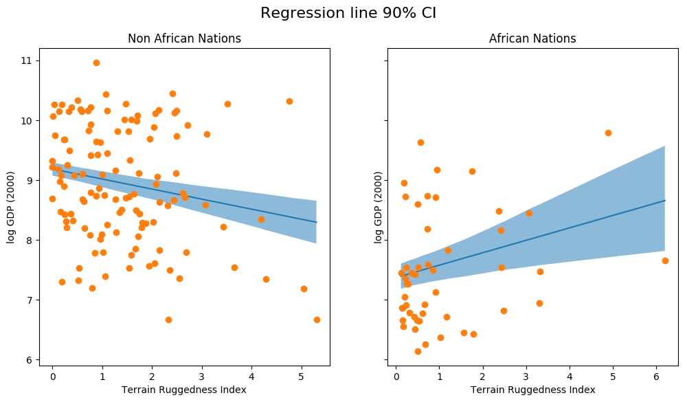
The above figure shows the uncertainty in our estimate of the regression line, and the 90% CI around the mean. We can also see that most of the data points actually lie outside the 90% CI, and this is expected because we have not plotted the outcome variable which will be affected by sigma! Let us do so next.
[17]:
fig, ax = plt.subplots(nrows=1, ncols=2, figsize=(12, 6), sharey=True)
fig.suptitle("Posterior predictive distribution with 90% CI", fontsize=16)
ax[0].plot(non_african_nations["rugged"],
           non_african_nations["y_mean"])
ax[0].fill_between(non_african_nations["rugged"],
                   non_african_nations["y_perc_5"],
                   non_african_nations["y_perc_95"],
                   alpha=0.5)
ax[0].plot(non_african_nations["rugged"],
           non_african_nations["true_gdp"],
           "o")
ax[0].set(xlabel="Terrain Ruggedness Index",
          ylabel="log GDP (2000)",
          title="Non African Nations")
idx = np.argsort(african_nations["rugged"])

ax[1].plot(african_nations["rugged"],
           african_nations["y_mean"])
ax[1].fill_between(african_nations["rugged"],
                   african_nations["y_perc_5"],
                   african_nations["y_perc_95"],
                   alpha=0.5)
ax[1].plot(african_nations["rugged"],
           african_nations["true_gdp"],
           "o")
ax[1].set(xlabel="Terrain Ruggedness Index",
          ylabel="log GDP (2000)",
          title="African Nations");
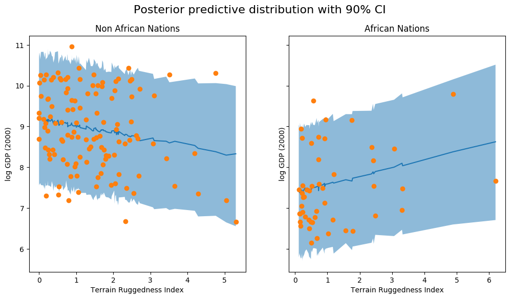
We observe that the outcome from our model and the 90% CI accounts for the majority of the data points that we observe in practice. It is usually a good idea to do such posterior predictive checks to see if our model gives valid predictions.
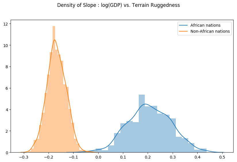
Finally, let us revisit our earlier question of how robust the relationship between terrain ruggedness and GDP is against any uncertainty in the parameter estimates from our model. For this, we plot the distribution of the slope of the log GDP given terrain ruggedness for nations within and outside Africa. As can be seen below, the probability mass for African nations is largely concentrated in the positive region and vice-versa for other nations, lending further credence to the original hypothesis.
[18]:
weight = samples["linear.weight"]
weight = weight.reshape(weight.shape[0], 3)
gamma_within_africa = weight[:, 1] + weight[:, 2]
gamma_outside_africa = weight[:, 1]
fig = plt.figure(figsize=(10, 6))
sns.distplot(gamma_within_africa, kde_kws={"label": "African nations"},)
sns.distplot(gamma_outside_africa, kde_kws={"label": "Non-African nations"})
fig.suptitle("Density of Slope : log(GDP) vs. Terrain Ruggedness");
Model Serving via TorchScript
Finally, note that the model, guide and the Predictive utility class are all torch.nn.Module instances, and can be serialized as TorchScript.
Here, we show how we can serve a Pyro model as a torch.jit.ModuleScript, which can be run separately as a C++ program without a Python runtime.
To do so, we will rewrite our own simple version of the Predictive utility class using Pyro’s effect handling library. This uses:
the
tracepoutine to capture the execution trace from running the model/guide code.the
replaypoutine to condition the sites in the model to values sampled from the guide trace.
[19]:
from collections import defaultdict
from pyro import poutine
from pyro.poutine.util import prune_subsample_sites
import warnings


class Predict(torch.nn.Module):
    def __init__(self, model, guide):
        super().__init__()
        self.model = model
        self.guide = guide

    def forward(self, *args, **kwargs):
        samples = {}
        guide_trace = poutine.trace(self.guide).get_trace(*args, **kwargs)
        model_trace = poutine.trace(poutine.replay(self.model, guide_trace)).get_trace(*args, **kwargs)
        for site in prune_subsample_sites(model_trace).stochastic_nodes:
            samples[site] = model_trace.nodes[site]['value']
        return tuple(v for _, v in sorted(samples.items()))

predict_fn = Predict(model, guide)
predict_module = torch.jit.trace_module(predict_fn, {"forward": (x_data,)}, check_trace=False)
We use torch.jit.trace_module to trace the forward method of this module and save it using torch.jit.save. This saved model reg_predict.pt can be loaded with PyTorch’s C++ API using torch::jit::load(filename), or using the Python API as we do below.
[20]:
torch.jit.save(predict_module, '/tmp/reg_predict.pt')
pred_loaded = torch.jit.load('/tmp/reg_predict.pt')
pred_loaded(x_data)
[20]:
(tensor([9.2165]),
 tensor([[-1.6612, -0.1498,  0.4282]]),
 tensor([ 7.5951,  8.2473,  9.3864,  9.2590,  9.0540,  9.3915,  8.6764,  9.3775,
          9.5473,  9.6144, 10.3521,  8.5452,  5.4008,  8.4601,  9.6219,  9.7774,
          7.1958,  7.2581,  8.9159,  9.0875,  8.3730,  8.7903,  9.3167,  8.8155,
          7.4433,  9.9981,  8.6909,  9.2915, 10.1376,  7.7618, 10.1916,  7.4754,
          6.3473,  7.7584,  9.1307,  6.0794,  8.5641,  7.8487,  9.2828,  9.0763,
          7.9250, 10.9226,  8.0005, 10.1799,  5.3611,  8.1174,  8.0585,  8.5098,
          6.8656,  8.6765,  7.8925,  9.5233, 10.1269, 10.2661,  7.8883,  8.9194,
         10.2866,  7.0821,  8.2370,  8.3087,  7.8408,  8.4891,  8.0107,  7.6815,
          8.7497,  9.3551,  9.9687, 10.4804,  8.5176,  7.1679, 10.8805,  7.4919,
          8.7088,  9.2417,  9.2360,  9.7907,  8.4934,  7.8897,  9.5338,  9.6572,
          9.6604,  9.9855,  6.7415,  8.1721, 10.0646, 10.0817,  8.4503,  9.2588,
          8.4489,  7.7516,  6.8496,  9.2208,  8.9852, 10.6585,  9.4218,  9.1290,
          9.5631,  9.7422, 10.2814,  7.2624,  9.6727,  8.9743,  6.9666,  9.5856,
          9.2518,  8.4207,  8.6988,  9.1914,  7.8161,  9.8446,  6.5528,  8.5518,
          6.7168,  7.0694,  8.9211,  8.5311,  8.4545, 10.8346,  7.8768,  9.2537,
          9.0776,  9.4698,  7.9611,  9.2177,  8.0880,  8.5090,  9.2262,  8.9242,
          9.3966,  7.5051,  9.1014,  8.9601,  7.7225,  8.7569,  8.5847,  8.8465,
          9.7494,  8.8587,  6.5624,  6.9372,  9.9806, 10.1259,  9.1864,  7.5758,
          9.8258,  8.6375,  7.6954,  8.9718,  7.0985,  8.6360,  8.5951,  8.9163,
          8.4661,  8.4551, 10.6844,  7.5948,  8.7568,  9.5296,  8.9530,  7.1214,
          9.1401,  8.4992,  8.9115, 10.9739,  8.1593, 10.1162,  9.7072,  7.8641,
          8.8606,  7.5935]),
 tensor(0.9631))
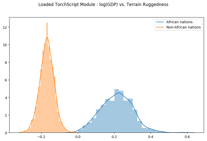
Let us check that our Predict module was indeed serialized correctly, by generating samples from the loaded module and regenerating the previous plot.
[21]:
weight = []
for _ in range(800):
    # index = 1 corresponds to "linear.weight"
    weight.append(pred_loaded(x_data)[1])
weight = torch.stack(weight).detach()
weight = weight.reshape(weight.shape[0], 3)
gamma_within_africa = weight[:, 1] + weight[:, 2]
gamma_outside_africa = weight[:, 1]
fig = plt.figure(figsize=(10, 6))
sns.distplot(gamma_within_africa, kde_kws={"label": "African nations"},)
sns.distplot(gamma_outside_africa, kde_kws={"label": "Non-African nations"})
fig.suptitle("Loaded TorchScript Module : log(GDP) vs. Terrain Ruggedness");
In the next section, we’ll look at how to write guides for variational inference as well as compare the results with inference via HMC.
References
McElreath, D., Statistical Rethinking, Chapter 7, 2016
Nunn, N. & Puga, D., Ruggedness: The blessing of bad geography in Africa”, Review of Economics and Statistics 94(1), Feb. 2012